
Mastering Recommendation Systems for Machine Learning Interviews
A clear, intuitive walkthrough of the models and metrics that separate strong candidates from everyone else.

Recommendation systems guide much of what users see online and have become essential to how companies drive engagement and revenue. They operate on large, noisy, mostly implicit behavioral data, which makes them very different from typical supervised learning problems. This is why interview that focus on recommender system can trip candidates up.
A candidate has to know how to work with sparse interactions, reason about user intent, handle scale, and choose models that match real product constraints. This blog will help you build that skill set. You will learn how recommendation problems are framed, how to evaluate them, and how major modeling approaches work, including popularity based methods, content based filtering, and collaborative filtering. By the end, you will know how to explain these concepts clearly, justify modeling choices, and answer interview questions with confidence and structure.
Foundations of Recommendation Systems
Every recommendation system starts with data. Some of this data is explicit, which means the user directly tells us what they think, such as giving a movie five stars or writing a review. Most real systems, however, rely on implicit data. This includes clicks, watch time, purchase history, or even items the user looked at but ignored. These behaviors do not express preference as clearly as a rating, but they are far more common and give the system many more signals to learn from. Recommenders also use information about users and items, such as product descriptions or user attributes, to fill in gaps. In practice this data can be messy, incomplete, and very large, which is why interviewers expect you to understand concepts like sparsity and noise.
Once you understand what data is available, the next step is to decide what problem you are trying to solve. Some systems try to predict a score, such as a rating or a probability of engagement. Many modern systems instead focus on ranking, which means producing an ordered list of items from most relevant to least relevant.
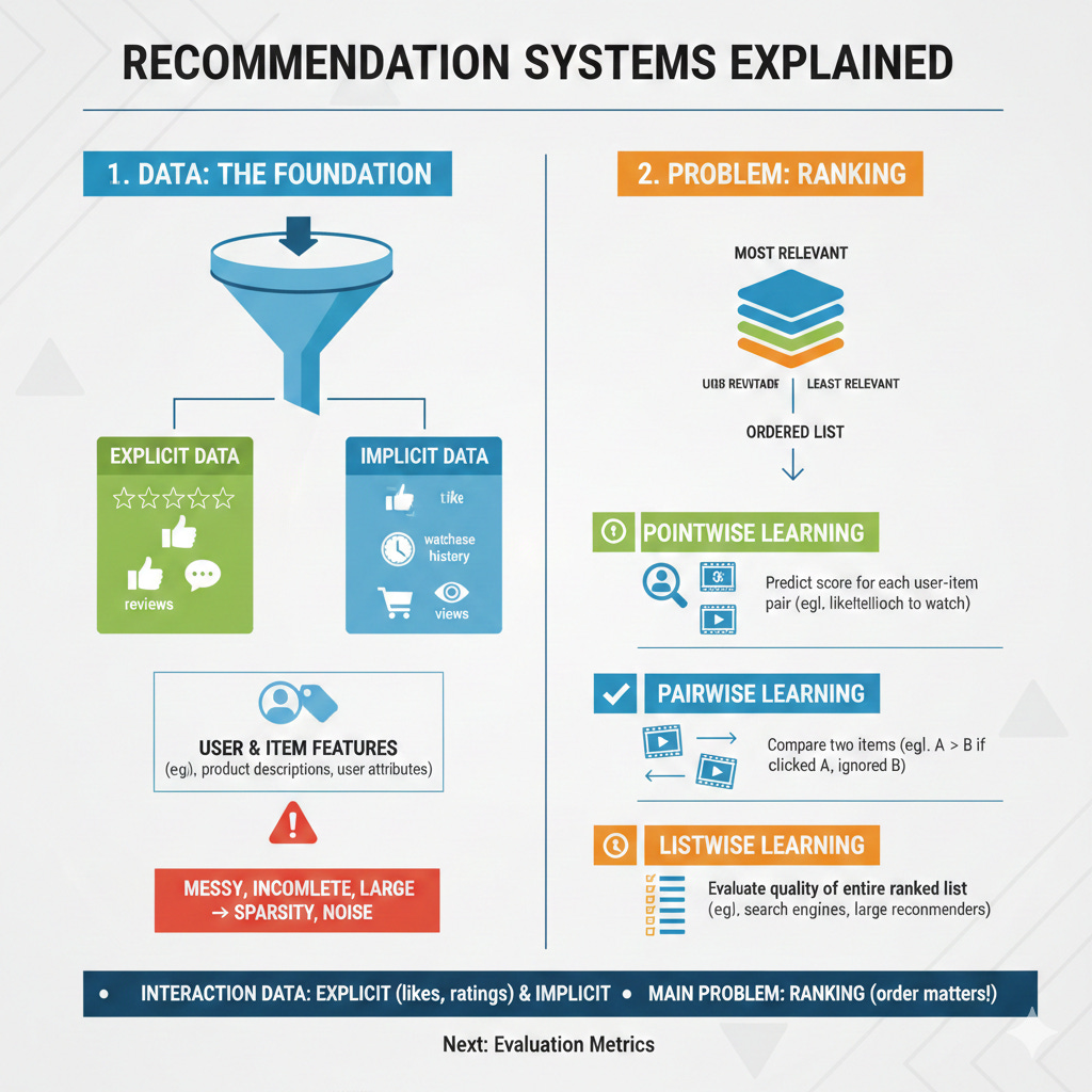
Ranking problems can be framed in different ways. One common approach is pointwise learning, where the model tries to predict a score for each user-item pair. For example, given a user and a movie, the model might predict how likely the user is to watch it. Pairwise learning takes a different view. Instead of predicting a score, it compares two items and decides which one the user prefers. For instance, if the user clicked Movie A but ignored Movie B, the model should rank Movie A higher. Listwise learning goes one step further. It evaluates the quality of an entire ranked list at once. Search engines and large scale recommenders often use listwise objectives because they directly optimize for producing a good ordered list rather than focusing on each item individually. Thinking about these three approaches helps you understand why different models behave differently and why ranking, not rating prediction, is usually the main goal.
Now it’s ok if you have a question about some of these topics (or all of them). We will dive into each over the next few blogs. The key things you need to remember are
Apart from user and item features, recommender system uses interaction data, and these interactions can be explicit (likes, ratings etc) or implicit (click, views, watch time, etc)
The machine learning problem we deal with here is not the typical regression, classification problem - rather its a ranking problem, where the order of the recommended items as predicted by the model is what we evaluate.
Now, before we move on to what ML models help solve the recommendation problem, let's first understand a bit more about the metrics that these model needs to optimize on.
Evaluation Metrics in Recommendation Systems
In a recommender system, the evaluation metrics are a bit different since model does not succeed simply because it predicts something. It succeeds when its predictions match what users find relevant, useful, and engaging.
Now, early recommendation systems treated recommendations are a regression problem, where they measured how close a model’s predicted rating is to the true rating provided by a user. The two most metrics used, understadably, at the time where RMSE and MAE. RMSE, or root mean squared error, penalizes larger mistakes more heavily. The formula is shown below.
A single large error increases RMSE significantly, which is why RMSE is sensitive to outliers. MAE, or mean absolute error, treats all mistakes the same regardless of their size.
MAE is easier to interpret and less influenced by rare extreme errors.
Although these metrics are useful for understanding prediction accuracy, they are less aligned with what most real recommendation systems care about. Many products do not even collect ratings, and even when they do, predicting a rating perfectly does not guarantee that the system will recommend the right items first.
For instance, a model that accurately predicts the rating for low-rated items (1- or 2-star), and inaccurately predicts the rating for high-rated items (4- or 5-star) can still have a low RMSE. But such a model would not make a good recommender system since it is unlikely to surface anything the user likes.
This is why ranking metrics dominate industry practice. Real systems must show the most relevant items at the top of a list, not simply predict the right score.
Precision at K and Recall at K
Precision at K and recall at K are the most common ranking metrics we use.
Precision at K measures how many of the top K recommended items are actually relevant to the user. If a system recommends ten items and four of them are relevant, the precision at K is forty percent. The formula below expresses this formally.
Recall at K measures how many of the relevant items the system successfully surfaced in the top K positions. If there are eight relevant items in total and the top ten recommendations include four of them, the recall at K is fifty percent.
These metrics are simple, easy to interpret, and commonly used in offline evaluation. However, they do not consider the order within the top K. In precision and recall at K, placing a relevant item in position one or in position ten counts the same. Real users behave differently. Items near the top receive far more attention. This limitation leads naturally to metrics that value early correctness more than late correctness.

Mean Average Precision
Mean average precision, usually written as MAP, improves on precision at K by rewarding models that place relevant items earlier in the list. Instead of treating all positions equally, MAP looks at the precision up to each position where a relevant item appears and averages these values. The idea is that a system should earn more credit if it finds the relevant items early rather than burying them deeper in the ranking.
Here, R is the total number of relevant items, P(i) is the precision at position i, and rel(i) is one if the item at position i is relevant and zero otherwise. MAP is the average of AP across all users.

By incorporating position in this way, MAP solves one weakness of precision at K. Yet MAP still treats each rank position independently and does not explicitly account for how attention drops off as users move farther down the list. In practice, users rarely scroll deeply, which motivates a metric that discounts lower positions more smoothly.
Discounted Cumulative Gain and Normalized Discounted Cumulative Gain
Discounted cumulative gain, or DCG, assigns higher value to relevant items that appear near the top and gradually reduces the reward for those that appear later. The discount factor is typically a logarithmic term, which reflects the idea that users strongly prefer top results and lose interest as they go down the list.

This formula captures a more realistic model of user attention. However, comparing DCG scores across users can be misleading. A user with many relevant items will naturally produce a higher DCG than a user with only a few. Normalized discounted cumulative gain, or NDCG, fixes this by dividing DCG by the ideal DCG, which is the score a perfect ranking would achieve for that user.
NDCG produces values between zero and one and is widely used in search and large scale recommendation systems because it captures position sensitivity while remaining comparable across users.
Metrics Beyond Accuracy and Ranking
Although ranking metrics measure how well the model orders items, real recommendation systems must also support business goals and user experience.
Coverage measures how much of the catalog is being recommended. A system with low coverage tends to show the same small set of items repeatedly, which may improve precision but reduces catalog exposure.
Diversity measures how different the recommended items are from each other. A common way to compute this is to take the average pairwise dissimilarity among all items in the recommendation list. If items are embeddings or represented with features, the dissimilarity can be one minus the similarity between item pairs.

A high diversity score means the list includes items from different categories or styles rather than many nearly identical items.
The main drawback is that maximizing diversity alone may harm relevance, since variety does not guarantee user interest.
Serendipity measures how pleasantly surprising the recommendations are. A recommendation is serendipitous if the user is likely to enjoy the item but the item is not something they would easily find on their own. A common version compares the recommended list to a simple baseline such as popularity, rewarding items that are relevant yet unexpected.

Here, B is a baseline recommendation set (often the top popular items), and rel(i) indicates whether item i is relevant to the user.
This metric rewards items that the baseline would not have recommended but that the user still likes. The downside is that serendipity depends heavily on the choice of baseline, and relevance labels may not always be available.
Novelty captures how unfamiliar or new the recommended items are to the user. A standard way to measure novelty is to use item popularity, assuming that less popular items are more novel. The most common formula uses the inverse log of item popularity.

Here, pop(i) is the probability of item i being interacted with in the global user base.
Recommending rare or long-tail items increases novelty. A disadvantage is that high novelty can surface irrelevant or obscure items that the user may not care about.
Business and Product Metrics
While accuracy and ranking metrics help us understand how well a model orders items, real recommendation systems are ultimately judged by whether they improve user behavior and business outcomes. Companies care about whether users click, purchase, stay engaged, or return to the platform over time.
The most common business metric is click-through rate, or CTR. This measures the fraction of recommended items that users click. If a system shows one hundred items and users click ten of them, the CTR is ten percent. In formula form, CTR is simply the ratio of clicks to impressions. A high CTR suggests that users find the recommendations interesting or relevant, but CTR has limitations. It only measures short term engagement and may reward clickbait or shallow interactions rather than meaningful consumption.
Conversion rate provides a deeper layer of insight, especially in ecommerce or subscription products. It measures the percentage of recommended items that lead to a purchase, subscription, or other target action. If a user sees twenty recommended items and buys one, the conversion rate is five percent. Conversion is harder to optimize because positive events are rare and influenced by many external factors, but it aligns more directly with business value. The drawback is that optimizing for conversion alone may push the system toward recommending only expensive or high margin items, which could reduce the overall user experience.
Most of these business metrics are evaluated not through offline experiments but through controlled online studies called A/B tests. In an A/B test, users are randomly split into two groups. One group receives recommendations from the current system and the other receives recommendations from the new model. By comparing CTR, conversion, or retention between the two groups, teams can isolate the effect of the recommendation algorithm with real users. A/B tests are widely used because offline metrics cannot perfectly predict what users will do in a live environment. However, A/B tests also require large traffic, careful statistical design, and enough time to reach stable conclusions (we will cover A/B tests in separate blog)
Now that we have a grasp of the metrics, let’s move into the models.
Popularity Based Recommendation Systems
Popularity based recommendation systems are the simplest kind of recommender, and they are often the first baseline used in both research and industry. The idea is straightforward. If many users interact with an item, then that item is likely to be appealing to new users as well. A system like this might recommend the most watched movies, the most purchased products, or the most clicked articles.
The strength of popularity based recommendations comes from the stability of collective behavior. Popular items tend to have many interactions, which reduces noise and makes their relative rankings easy to estimate. This is why popularity works well when a platform is new or when a user has no history. A cold start user who just signed up still sees reasonable content because the system does not need any personal information to make a recommendation. This idea is used by major platforms in areas like trending content sections. It ensures that the system always has something reasonable to show.
Although popularity is easy to compute, it has important limitations. Because the system recommends what is already receiving the most attention, it tends to reinforce the same small set of well known items. This creates what is often called a head tail imbalance. The most popular items gain more exposure, while less popular items remain hidden. For example, a small independent movie will almost never appear in a popularity based ranking, even if certain users might love it. This means the system provides no personalization. Every user sees the same set of items, regardless of their interests.
To make popularity based recommendations more useful, systems often introduce adjustments. One common improvement is segmented popularity. Instead of computing popularity across all users, the platform might compute popularity within a region, age group, or time window. This creates more relevant recommendations because popularity patterns differ across groups. Another improvement is temporal decay. A recent interaction is usually more meaningful than an older one, so the system may assign more weight to items that are currently trending. This helps the model adapt when user interest shifts quickly.
Even with these improvements, popularity methods still suffer from the central problem of lacking personalization. They can boost engagement in the short term by showing crowd favorites, but they do not help users discover the long tail of the catalog. This limitation is why popularity approaches often serve as the starting point rather than the final solution. Understanding how they work and where they break down is essential as we move toward more advanced methods like content based filtering and collaborative filtering. In interviews, discussing popularity based models shows that you understand the importance of baselines, the challenges of cold start, and the limits of non personalized recommendations.
Content Based Recommendation Systems
Content based recommendation systems take a very different approach from popularity based methods. Instead of assuming that items with many interactions are good for everyone, a content based system tries to understand what each item is about and what each user tends to prefer. The main idea is simple. If a user likes certain types of items, the system should recommend other items that share similar characteristics. This approach creates personalization without relying on other users’ behavior, which makes it especially powerful in situations where user interaction data is limited.

The foundation of a content based system is how it represents items. Every item must be converted into a feature vector that captures its key attributes. For text items such as news articles or product descriptions, these features might come from word frequency counts, TF IDF scores, or modern embedding models that produce dense vector representations. For movies or songs, features might come from genre labels, keywords, audio descriptors, or even deep learning models trained on raw content. Regardless of the method, the goal is to express each item in a form that allows the system to measure similarity between items.
Once items have feature representations, the next step is to create a profile for each user. A user profile captures the types of items the user has interacted with in the past. In simple systems, this profile might be the average of the feature vectors of all items the user liked. In more advanced systems, user profiles can be learned through models that weigh certain interactions more heavily or detect deeper patterns in the user’s behavior. The idea remains the same. A user profile summarizes what the user tends to enjoy in a way that can be compared directly with new items.
With user and item representations in place, the system ranks items by measuring how similar each item is to the user profile. A common approach is cosine similarity, which measures how closely two vectors align. If a user has watched several science fiction movies, the user profile will lean in that direction. The system will then identify other movies with similar feature representations and rank them higher. This flow creates a personalized experience even if the user has interacted with only a small number of items.
Content based systems come with clear strengths. They handle the item cold start problem well because they can recommend new items as long as those items have features. For example, a newly released movie can be recommended on day one because the system can analyze its description, genre, or poster. They also provide transparency. It is easy to explain why an item was recommended because the recommendation directly reflects shared content features.
However, content based methods also have limitations. Since the system recommends only items that are similar to what the user already liked, it may over specialize. A user who reads one science fiction book may be shown only science fiction going forward, even if they have other interests. This issue arises because the system does not learn from the broader behavior of other users. It cannot detect that people who enjoy science fiction also tend to enjoy certain thrillers or dramas. This type of cross preference learning requires stepping beyond content alone, which is where collaborative filtering becomes more powerful.
Despite these limitations, content based methods remain an essential part of many recommendation pipelines. They provide personalization early in a user’s lifecycle, work well with rich item metadata, and serve as strong candidates in the retrieval stage of large systems. Understanding how they work helps you explain the strengths and weaknesses of different modeling choices in interviews and prepares you for the next major technique, collaborative filtering, which learns from collective user behavior rather than content features.
Collaborative Filtering
Collaborative filtering is one of the most influential ideas in recommendation systems. Unlike content based methods, which rely on item features, collaborative filtering learns from the collective behavior of users. The key idea is simple. If two users behave similarly, then items liked by one user are likely to be relevant to the other. Similarly, if two items are liked by many of the same users, those items are probably similar. This ability to learn directly from patterns in the interaction data makes collaborative filtering extremely powerful once the system has enough user behavior to analyze.
The most direct form of collaborative filtering is user based collaborative filtering. This method tries to identify users who have similar tastes. To make this concrete, imagine a matrix where each row is a user and each column is an item. A value in the matrix might represent a rating or an implicit signal like a click or a purchase. To find users with similar preferences, the system looks at their interaction patterns. A common way to measure similarity is cosine similarity. If we represent two users as vectors of their interactions with items, cosine similarity measures the angle between these vectors.
If two users have interacted with many of the same items, their vectors will align and the similarity score will be high. Once the system identifies a set of similar users, it can recommend items that these similar users interacted with but the target user has not yet engaged with. This approach creates personalization without requiring any item metadata. The main challenge is that user behavior can be sparse, meaning the overlap between two users often contains very few items. When that happens, the similarity estimate becomes unreliable.
, such that the dot product of the two embeddings approximates the ground truth value in the feedback matrix.")
Item based collaborative filtering solves this sparsity issue by flipping the perspective. Instead of comparing users to each other, we compare items to each other. Two items are considered similar if many of the same users interacted with both. For example, if many users who watched one science fiction movie also watched another, those two movies will have a high similarity score. We can compute this with the same cosine similarity formula but applied to item vectors.
Item based collaborative filtering uses these similarities to recommend items that are closest to the ones a user already interacted with. If a user watched a particular movie, the system retrieves movies that are similar to that specific item. This approach produces stable recommendations because item vectors tend to be denser and less volatile than user vectors. Users often interact with only a small number of items, but popular items may be interacted with by thousands of users, which improves the quality of similarity estimates.
A simple example helps make this concrete. Suppose a user has watched Movie A and Movie B. The system computes similarities between these movies and all other movies. If Movie C has high similarity with Movie A and Movie D has high similarity with Movie B, the system can combine these similarity scores to rank Movies C and D for the user. A common scoring method is a weighted sum of similarities.
Here, Items(u) represents the set of items the user has interacted with. An item receives a higher score if it is strongly similar to several items the user already liked. This simple scoring formula forms the basis of item based collaborative filtering in many real systems.
Item based collaborative filtering is widely used in industry because of its stability and scalability. A classic example comes from Amazon, which found that item item similarities worked better than user user similarities in large scale environments. Items change slowly over time, while user behavior can be unpredictable and sparse. Computing a similarity matrix for items once and updating it periodically is much easier than constantly recomputing similarities between millions of users. This makes item based collaborative filtering efficient while still producing high quality personalized recommendations.
Although collaborative filtering is powerful, it does depend on having enough interaction data. If no users have interacted with a new item, the system cannot compute similarities for it. This is known as the item cold start problem. Conversely, new users with only a few interactions may also receive poor recommendations because the system cannot accurately determine their preferences. These limitations motivate more advanced methods like matrix factorization, which extract deeper patterns from sparse data.
Collaborative filtering represents a major shift in how we think about recommendations. Instead of requiring content features or domain knowledge, the system learns patterns directly from the behavior of many users. This ability to leverage collective intelligence is why collaborative filtering remains a core technique in both academic research and industrial recommendation systems. Understanding user based and item based collaborative filtering is the foundation for more advanced models that we will explore in the next sections.
Matrix Factorization
Matrix factorization is one of the most important ideas behind modern recommendation systems. It builds on the intuition of collaborative filtering but goes deeper by trying to uncover hidden patterns that explain why users interact with certain items. Instead of comparing users or items directly, matrix factorization assumes that user behavior can be explained by a smaller set of underlying factors. These factors are not labeled explicitly but are learned from the interaction data. For example, a movie might appeal to users who like complex characters, fast paced action, or emotional storylines. These qualities are not written anywhere in the data, but matrix factorization can still learn them automatically.

The basic setup starts with a user item interaction matrix, where each row represents a user, each column represents an item, and each entry represents a rating or some form of implicit feedback. This matrix is usually extremely sparse because any user interacts with only a tiny fraction of the catalog. The goal of matrix factorization is to represent each user and each item as vectors in a lower dimensional space. If the user matrix is called U and the item matrix is called V, then the predicted interaction between a user and an item is the dot product between their vectors. The mathematical formulation looks like the expression below.
Here, u is the latent factor vector for user u, and vi is the latent factor vector for item i. The model learns these vectors by minimizing the difference between the predicted interactions and the true interactions. A common objective function used during training is shown below.
The set Ω contains all user item pairs where feedback is observed. This approach captures preference patterns even when there is no obvious content feature linking items together. If two items appeal to similar types of users, their vectors will naturally end up close to each other in the latent space.
One of the biggest advantages of matrix factorization is its ability to handle sparsity. In user based or item based collaborative filtering, you need enough overlap between users or items to compute similarity scores reliably. Matrix factorization does not require direct overlap. It can learn meaningful user and item vectors even when most entries in the interaction matrix are missing. This is possible because the model uses all the data simultaneously to infer the latent structure. As long as enough users and items share some indirect links through patterns in the data, the factors will align in a way that produces good predictions.
Another strength of matrix factorization is interpretability at the conceptual level. Although we do not assign explicit meanings to the latent dimensions, they often correspond to intuitive properties. A user vector might represent degrees of preference for genres, themes, or styles, while an item vector might represent how strongly the item expresses those qualities. A high dot product between the vectors suggests that the user is likely to enjoy the item. This interpretation helps when explaining the model in interviews because you can describe recommendations in terms of matching user preferences to item characteristics, even if those characteristics are learned rather than hand engineered.
Matrix factorization also provides a natural way to incorporate additional modeling tricks. Bias terms account for the fact that some users give higher ratings in general, while some items are broadly liked regardless of user preference. Implicit feedback extensions modify the objective to better capture what clicks or views mean. Techniques like alternating least squares and stochastic gradient descent make training efficient at large scale. These extensions allow the same core idea to adapt to real world platforms with millions of users and items.
The main limitations of matrix factorization come from its assumptions. It struggles with cold start problems because new users and items have no learned vectors until they generate interactions. It also assumes that user preferences can be represented by a relatively small number of latent factors, which may not capture very complex behavior. Even so, matrix factorization remains a foundational technique because it offers a balance of accuracy, scalability, and conceptual clarity. It is one of the most widely discussed methods in interviews, and understanding it prepares you to learn more advanced approaches such as neural recommendation models and sequence based techniques.
Core Techniques
Matrix factorization models can be trained in several different ways, and each method reflects a slightly different view of how user preferences should be represented. One of the earliest approaches comes from the standard singular value decomposition, or SVD. In classical linear algebra, SVD decomposes a matrix into three components that capture its essential structure. However, the user item interaction matrix in recommendation systems is almost always sparse, with most entries missing. Because classical SVD requires a complete matrix, it cannot be applied directly. Instead, researchers developed adapted versions of SVD that focus only on the observed entries and learn low dimensional user and item vectors that reconstruct these values well.

A major improvement to basic SVD is SVD plus plus, also written as SVD++. This technique was developed during the Netflix Prize and became well known because of how effectively it handled implicit feedback. The idea behind SVD++ is that every user is influenced not only by the items they rated but also by the items they interacted with in weaker ways, such as clicks or views. By including these implicit interactions in the user representation, SVD++ learns richer user vectors and produces better recommendations. This makes the method especially useful in modern platforms where explicit ratings are rare and almost all signals come from behavior.
To train matrix factorization models efficiently, many systems use alternating least squares, or ALS. ALS approaches the factorization problem by fixing one set of vectors and solving for the other in a closed form, then switching roles and repeating the process. When the item vectors are fixed, each user vector can be solved independently, and when the user vectors are fixed, each item vector can be solved independently. This alternating structure makes ALS naturally parallelizable, which is why it is often used in large scale environments such as Spark based pipelines. ALS is especially popular when the focus is on implicit feedback datasets, because it can be adapted to weight different types of interactions differently.
Another widely used optimization method is stochastic gradient descent, or SGD. Instead of solving for user and item vectors in closed form, SGD updates the vectors gradually by following the gradient of the loss function. Each observed interaction provides a small correction to the user and item vectors involved. Over time, these repeated updates lead the model toward a configuration that predicts interactions accurately. SGD is flexible, easy to implement, and works well with a variety of loss functions and regularization terms. It is also the method most often used in research and industry when experimenting with new variants of matrix factorization, because it integrates smoothly with additional model components.
All of these training techniques rely on the idea of preventing overfitting. If the user and item vectors become too specialized to the training data, the model may perform poorly on new interactions. Regularization helps control this by adding a penalty for large vector values, encouraging the model to learn general patterns rather than memorize specific observations. Whether using ALS or SGD, regularization is a crucial part of achieving stable and reliable matrix factorization models.
Together, SVD based approaches, ALS, and SGD form the core toolkit for building matrix factorization models. They reflect different tradeoffs between accuracy, scalability, and implementation complexity. Understanding these methods makes it easier to discuss how real recommendation systems are trained, how they scale to millions of users and items, and how you might choose the right technique in an interview scenario.
How to Choose Between Recommendation Models
Choosing the right recommendation approach depends on how much data is available, how diverse that data is, how quickly you need the system to scale, and what each product values most. Different methods make different assumptions about user behavior, and those assumptions only work when the underlying data supports them. A system with abundant interaction history can lean on collaborative filtering because patterns of co-consumption become reliable. But when the data is sparse and most users have interacted with only a handful of items, collaborative filtering becomes unreliable, and content-based approaches or even simple popularity models may outperform it. Cold start severity also plays a large role. If new users arrive frequently and provide very little initial signal, a popularity model or a content-based model may serve as a safer starting point until enough behavior accumulates. Similarly, if the catalog grows quickly with new items appearing constantly, a content-based model that learns from item attributes becomes necessary because collaborative filtering has no behavioral data to learn from for such items.
Scale influences these choices in a subtler way. Some methods, such as memory-based nearest-neighbor approaches, become expensive when the user base or catalog grows very large. They work well for smaller systems but eventually struggle with latency and compute constraints. Matrix factorization and embedding-based methods scale more naturally because they compress users and items into fixed-dimensional vectors. At massive scale, retrieval architectures become essential. Large recommender systems often start with approximate nearest-neighbor search to retrieve a manageable candidate set, since ranking all items directly is infeasible. The available computational budget and latency constraints guide which models can be used in the retrieval stage and which belong in the ranking stage. Business goals refine these decisions further. A news platform may optimize for freshness and diversity, while an e-commerce platform may care more about precision at the top of the list or long-term value. A system designed to maximize conversions may favor methods that exploit behavioral signals even if they require heavy modeling complexity, while a system emphasizing discovery may incorporate more content-driven or diversity-driven components.
In practice, most production systems do not choose a single method but instead assemble hybrids that combine the strengths of several approaches. A common pattern is a two-stage architecture consisting of retrieval and ranking. Retrieval focuses on efficiently pulling a few hundred candidates from a large catalog. This stage may rely on simple models such as popularity, embedding similarity, or lightweight collaborative filtering, because speed matters more than perfect ranking accuracy. The ranking stage is more expressive and can use richer models such as gradient-boosted trees, deep neural rankers, or hybrid scoring functions. The idea is to let the retrieval stage filter broadly and then let the ranking stage apply a more detailed relevance model.
Common Interview Questions
Why are ranking metrics preferred over rating prediction metrics?
Rating metrics like RMSE treat all prediction errors equally, including errors on items the user will never see. Ranking metrics evaluate whether the most relevant items appear early in a list, which aligns directly with user experience. A model with low RMSE can still produce poor rankings, while strong ranking metrics reliably reflect actual recommendation quality.
Why is collaborative filtering effective?
Collaborative filtering captures patterns of co-consumption. Users who behave similarly toward items tend to share preferences even without item metadata. This allows the system to learn rich preference structures from interaction data alone. Once enough users and interactions exist, collaborative filtering often outperforms content-based methods because it models preference behavior directly.
Why is item–item collaborative filtering often preferred over user–user?
Item similarity tends to be more stable because items change slowly over time, while user behavior can be noisy and inconsistent. Item–item similarity is easier to scale: the number of items is usually much smaller than the number of users, and item vectors remain meaningful even for new users. This stability makes item-based CF more reliable in production.
How do you handle cold start for new users?
Use methods that do not rely on behavioral history. Popularity-based recommendations provide a safe default. Content-based recommendations use user-provided attributes, onboarding surveys, or contextual features. As soon as the user generates meaningful interactions, the system can gradually introduce collaborative filtering.
How do you handle cold start for new items?
Collaborative models cannot recommend items with no interaction data. Content-based models can describe new items using metadata, text, or learned embeddings. You can also boost exposure for new items so they gather initial interactions, after which CF models incorporate them naturally.
What is the advantage of matrix factorization over memory-based CF?
Matrix factorization generalizes better under sparsity and scales more efficiently. It learns latent representations of users and items, smoothing noise and filling missing entries. Memory-based methods rely directly on observed interactions and become unstable when user histories are short or inconsistent.
What are the weaknesses of popularity-based recommendation?
It has no personalization and reinforces exposure toward already popular items. It fails for niche users and contributes to filter bubbles. However, its strength is stability and cold-start robustness, which makes it a useful fallback.
How do you evaluate a recommender trained with implicit feedback?
Use ranking metrics such as Precision@K, Recall@K, MAP, or NDCG. Construct positive labels from interactions and treat non-interacted items as uncertain negatives. Sampling strategies for negatives become critical. Offline metrics should eventually be validated through online A/B testing since implicit relevance labels are imperfect.
Why do we need negative sampling in implicit-feedback models?
Implicit data does not contain explicit negatives. Treating all missing interactions as negatives produces huge class imbalance and misleading gradients. Negative sampling provides a tractable, meaningful approximation of non-preference and stabilizes learning.
How do approximate nearest neighbor methods help in large-scale retrieval?
ANN algorithms speed up similarity search by trading tiny amounts of accuracy for much lower latency. They are necessary because finding nearest neighbors exactly in high dimensions is too slow. ANN enables retrieving hundreds of candidates from millions of items in real time, forming the first stage of most large recommendation pipelines.
What tradeoff exists between content-based and collaborative filtering?
Content-based models excel at cold start and interpretability but may over-personalize and limit discovery. Collaborative filtering captures behavioral patterns but requires sufficient interaction data and struggles with new users or new items. Many systems use hybrids to balance these tradeoffs.
What are the challenges with implicit negative signals?
A lack of interaction does not guarantee disinterest. Users may not see the item, may not browse long enough, or may have been saturated with similar content. Treating every non-interaction as a negative label can bias models heavily. This ambiguity requires specialized loss functions and evaluation strategies.
Why is diversity important in a recommendation list?
Even accurate recommendations can feel repetitive if they are too similar. Diversity improves user satisfaction, prevents overfitting to short-term behavior, and encourages exploration. It is especially important in domains where users consume multiple items in sequence, such as streaming or news.
How do you prevent a recommender from overfitting?
Use regularization in matrix factorization, dropout in deep models, temporal validation splits, and constraints such as limiting co-occurrence-based memorization. More importantly, evaluate on realistic datasets and verify generalization through online metrics, since recommender overfitting often appears only in deployment.
How do you choose which evaluation metric to optimize?
The choice depends on the product’s structure. Small carousels value Precision@K because only the top few items matter. Long feeds benefit from NDCG because it models graded relevance and attention decay. Search-like systems emphasize MRR because the first correct match dominates. Always tie metric choice to user experience and business goals.
Final Takeaways
A strong understanding of recommendation systems comes from recognizing how each modeling approach, evaluation metric, and design decision fits into the broader landscape of user behavior and system constraints. The foundation begins with data. Real recommendation systems rely heavily on implicit feedback, which is abundant but noisy. This shifts the problem away from predicting precise ratings and toward ranking items effectively. Understanding this shift explains why RMSE is insufficient on its own and why ranking metrics such as Precision@K, Recall@K, MAP, and NDCG better reflect what users actually experience. It also explains why different metrics emerged over time, each addressing limitations in the ones that came before it.
The modeling methods themselves each serve distinct roles. Popularity-based recommendations provide stable, cold start friendly baselines. Content-based systems capture item attributes and help surface meaningful suggestions even when interaction history is scarce. Collaborative filtering harnesses collective behavioral patterns once enough data accumulates and often becomes the backbone of personalization. Knowing when each method works and when it fails is one of the most important interview skills, especially when you are expected to reason about cold start challenges, sparsity, scale, and catalog growth.
Throughout all of this, tradeoffs matter. A system optimized purely for accuracy may fail on diversity or novelty. A model designed for perfect ranking may fail to scale. Techniques that excel with rich user histories may collapse under cold start pressure. Interviewers want to see that you can balance these competing forces and justify choices based on product goals, data realities, and performance constraints. This ability to reason through alternatives is ultimately more important than knowing any single algorithm in isolation.
Really thorough walkthrogh of the recsys landscape. The pointwise vs pairwise vs listwise framing is particulary insightful, it clarifies why item-based CF stabilizes better than user-based in production. What I found especially valuable is the two-stage retrieval/ranking architecture discussion, since most interview prep materials skip over how these systems actualy scale. The observation that item vectors tend to be denser than user vectors becuase popular items get thousands of interactions explains a lot about why item-item similarities work better at scale.