
Data Science Interview Guide - Part 7: kNN
Why are interviewers asking questions about a model rarely used in production?

k Nearest Neighbors is not one of the most frequently asked machine learning interview topics. Many interviews will never mention it at all. When it does appear, however, it is almost never because the interviewer cares about kNN as a production model.
kNN shows up because it is simple. That simplicity makes it a useful tool for probing whether a candidate understands foundational concepts rather than memorized formulas. With very little setup, an interviewer can test how you reason about similarity, distance, feature scaling, bias variance tradeoffs, and computational cost.
In this blog, you will get to learn exactly this - through the lens of kNN. How kNN makes predictions for both classification and regression, how the choice of distance metric and the value of k affect model behavior, and why preprocessing steps such as feature scaling are not optional. You will also understand why kNN struggles in high dimensional spaces, how it can be optimized using indexing and approximate nearest neighbor methods, and when it is appropriate to use kNN in practice.
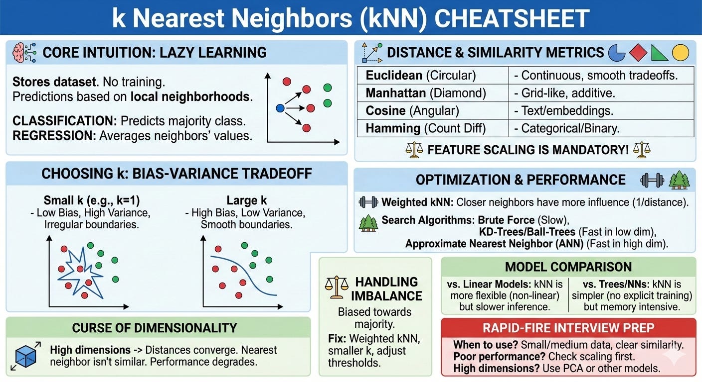
Core Intuition: How kNN Works
k Nearest Neighbors starts from a single assumption. If two data points are similar, their outputs should also be similar. Instead of trying to learn a global rule from the data, kNN keeps the data as it is and reasons directly from it when a prediction is needed.
Because of this, the training phase is almost trivial. The model simply stores the dataset. The real work happens at prediction time, when a new data point arrives and the algorithm asks a very direct question. Which existing points look most like this one.
To see how this works in practice, consider a simple house price prediction problem. Each house is represented by features such as square footage and number of bedrooms. When a new house appears, kNN computes its distance to every house in the training set. It then selects the k closest houses and uses their prices to form a prediction. If the nearby houses sold for similar prices, kNN assumes the new house should as well.
This process does not change depending on whether the task is classification or regression. In a classification setting, kNN looks at the labels of the nearest neighbors and predicts the most common one. In a regression setting, it aggregates the neighbors’ target values, typically by taking their average. In both cases, the core operation is the same. Find the nearest points, then combine their outputs.
The idea of “nearest” depends entirely on how distance is defined. Distance is computed between feature vectors using a chosen metric, and that metric determines what it means for two points to be similar. If features are on very different scales, the largest scale feature will dominate the distance calculation and distort the neighborhood structure. This is why feature scaling is essential for kNN and why preprocessing directly affects its behavior.
Because kNN bases its predictions on small neighborhoods rather than the entire dataset, it is a local method. Each prediction is influenced only by nearby points. This allows kNN to adapt to complex patterns without learning an explicit model, but it also makes the algorithm sensitive to noise and to how densely the data is distributed.
Understanding kNN is ultimately about understanding this flow. A new point arrives, distances are computed, neighbors are selected, and their outputs are combined. If you can explain this sequence clearly and relate it to the geometry of the data, you understand the core of kNN and can answer most interview questions about it.

Distance the Similairty Metrics
At the heart of k Nearest Neighbors is a single question. How do we decide whether two points are similar. The answer to that question is the distance or similarity metric, and this choice has a larger impact on kNN than almost any other design decision.
kNN does not learn which features matter more or how they should interact. It follows the geometry defined by the distance function you choose. If that geometry does not reflect the structure of the data, kNN will confidently select the wrong neighbors.
Lets continue with the house price example, where each house is represented by square footage and number of bedrooms. Imagine plotting these houses on a two dimensional plane. The distance metric you choose determines the shape of the neighborhoods around each point.
With Euclidean distance, neighborhoods are circular. All points lying on a circle around a house are considered equally similar, even if they differ in very different ways across the two features. A house that is slightly smaller but has more bedrooms can be considered just as similar as one that is larger with fewer bedrooms, as long as the overall straight line distance is the same. This reflects an assumption that deviations in different features can trade off smoothly against each other.
Manhattan distance creates a different geometry. Neighborhoods become diamond shaped rather than circular. Distance grows by moving along each feature independently, rather than diagonally through the space. In this geometry, large changes in one feature cannot be fully compensated by small changes in another. This often makes Manhattan distance feel more intuitive when features contribute additively and independently to similarity.
This geometric difference is what interviewers care about. The formulas are simple. The implications of those formulas for neighborhood structure and decision boundaries are not.
Cosine similarity changes the notion of similarity even more dramatically. It ignores absolute distance and focuses only on direction. Two points can be very far apart in magnitude and still be considered similar if they lie along the same direction from the origin. This is why cosine similarity is so effective for text and embedding based representations, where the relative pattern of features matters more than their scale.
Hamming distance applies when features are categorical or binary. Instead of measuring how far apart two points are, it counts how many features differ. This highlights an important principle that interviewers often probe. The distance metric must match the type of data. Applying a continuous distance to categorical features usually produces meaningless neighborhoods.
 Algorithm | by Thant Thiri Maung | Medium")
All distance metrics encode assumptions about similarity. kNN does not adapt or correct those assumptions. It enforces them exactly.
This is also why feature scaling and distance choice are inseparable in kNN. Scaling changes the shape of the space, which changes which points fall into a neighborhood. A simple rescaling of features can completely change the set of nearest neighbors and therefore the prediction.
When interviewers ask about distance metrics, they are testing whether you can reason about the geometry induced by those metrics and explain how that geometry affects model behavior.
Choosing k: Bias Variance Tradeoff
Once a distance metric is chosen, the most important remaining decision in k Nearest Neighbors is the value of k. This single number controls how much local information the model uses when making a prediction, and it has a direct and intuitive connection to the bias variance tradeoff.
To understand this, return to the house price example. Imagine predicting the price of a new house using only the single closest neighbor. The prediction will closely follow the nearest observed example. If that neighbor happens to be noisy or unusual, the prediction will be noisy as well. The model is highly flexible and very sensitive to small changes in the data.
This is the low bias, high variance regime. The model can adapt to fine details in the data, but its predictions are unstable and can change dramatically if the dataset changes slightly.
Now imagine increasing k so that the prediction is based on many nearby houses. Individual quirks in any one house matter less, because they are averaged out by the larger neighborhood. The prediction becomes smoother and more stable.

This moves the model toward higher bias and lower variance. The model becomes less sensitive to noise, but it also loses the ability to capture sharp local patterns. If the true relationship between features and price changes rapidly in different regions of the space, a large k will blur those differences.
The value of k controls the size of the neighborhood that defines similarity. Small k means very local decision making. Large k means more global averaging. In practice, k is usually chosen through cross validation. The goal is not to find a universally correct value, but one that balances stability and flexibility for the specific dataset and distance metric being used.
When interviewers ask about choosing k, they are testing whether you understand how this single parameter controls model behavior. If you can explain how k changes sensitivity to noise, smoothness of decision boundaries, and generalization, you are answering the question at the level they expect.
The Curse of Dimensionality Catch
As the number of features grows, distance in k Nearest Neighbors starts to behave in a counterintuitive way. Each feature introduces another opportunity for two points to differ. Even if the difference along any single feature is small, those differences accumulate.
Imagine comparing two houses using just square footage. A difference of a few hundred square feet might feel meaningful but manageable. Now add bedrooms. Add age of the house. Add distance to city center. Add number of bathrooms. Add school rating. Each of these adds a small difference. On its own, none of these differences is dramatic.
But kNN adds all of them together.
As the number of features increases, these small differences keep stacking up. Eventually, every house differs from every other house in many small ways. The total distance between any two houses becomes large, not because they are extremely different in one aspect, but because they are slightly different in many aspects.
This is where the problem begins. If you look at the distances from a new house to all houses in the dataset, they will all be large, and more importantly, they will all be similar in magnitude. The nearest house is no longer meaningfully near. It is simply the one with the smallest sum of many small differences.
From the perspective of kNN, this makes it very hard to decide what is truly similar. The algorithm still ranks neighbors by distance, but the difference between the closest neighbor and the farthest neighbor becomes small relative to the total distance. Distance loses its ability to separate good neighbors from bad ones.
Adding more data does not fully solve this problem. As dimensionality increases, you would need exponentially more data to find points that are genuinely close across most dimensions. In practice, that amount of data is rarely available.
When interviewers talk about the curse of dimensionality in kNN, this is the intuition they are looking for. In high dimensions, small differences add up, distances become large and similar, and nearest neighbors stop being meaningfully similar.
Optimizing kNN for Real World Use
Feature Scaling
kNN makes decisions purely based on distance. If features live on different numerical scales, the feature with the largest range will dominate the distance calculation. This domination is not subtle. Even small differences in a large scale feature can completely outweigh meaningful differences in smaller scale features.
Consider again the house price example. If square footage ranges in the thousands and the number of bedrooms ranges from one to five, Euclidean distance will be driven almost entirely by square footage. Two houses with identical size but very different layouts will appear more similar than two houses with nearly identical layouts but slightly different sizes. The algorithm is not making a modeling choice here. It is simply obeying the units of measurement.
Standardization is commonly used to address this problem. By centering each feature and scaling it to unit variance, differences across features become comparable in relative terms. Normalization, where features are scaled to lie within a fixed range such as zero to one, is often preferred when features have natural bounds or heavy tails. The exact method is less important than the outcome. No single feature should dominate distance purely because of its scale.
Scaling becomes even more important when working with heterogeneous features. Real world datasets often mix continuous features, counts, binary indicators, and sometimes encoded categorical variables. Applying a single distance metric across such features without careful scaling almost always leads to distorted neighborhoods. In these settings, scaling is effectively how you express feature importance in kNN.

From an interview perspective, the key point is simple. kNN does not learn feature weights. Feature scaling is how you control which features matter. Without it, nearest neighbors are determined by units, not by meaning.
Weighted kNN
So far, k Nearest Neighbors has treated all neighbors as equally important. Once the k nearest points are identified, each of them contributes the same weight to the final prediction. This is known as uniform voting in classification and uniform averaging in regression. While simple, this approach makes a strong assumption that all neighbors within the chosen neighborhood are equally informative.
In practice, this assumption is often too crude. Even within a small neighborhood, some points are clearly more similar to the query than others. A house that is almost identical in size and layout should influence the prediction more than one that barely made it into the top k.
Weighted kNN addresses this by assigning more influence to closer neighbors and less influence to farther ones. The most common approach is inverse distance weighting, where each neighbor’s contribution is proportional to the inverse of its distance from the query. Points that are very close receive large weights, while points near the edge of the neighborhood receive much smaller weights.
This changes how predictions behave. In classification, closer neighbors effectively get more votes, which can help resolve ambiguous cases where uniform voting might be dominated by several marginal neighbors. In regression, the prediction becomes a weighted average that is pulled toward the most similar points rather than treating all neighbors equally.
One of the main benefits of weighted kNN is improved robustness to noisy data. Noise often appears as isolated or weakly related points that happen to fall within the neighborhood. Under uniform voting, these noisy neighbors can have as much influence as genuinely similar points. With distance based weighting, their impact is naturally reduced because they tend to lie farther from the query.
Weighted kNN also softens the sensitivity to the exact choice of k. When k is slightly too large, uniform kNN may include neighbors that dilute the signal. Weighted kNN reduces this effect by down weighting those marginal neighbors, allowing the closest points to dominate the prediction.
From an interview perspective, the key insight is that weighted kNN does not change how neighbors are selected. It changes how much each neighbor matters.
Making Search Faster
Vanilla kNN uses what we call Exact Nearest Neighbour Search - where we guarantee finding the true nearest neighbors according to the chosen distance metric. For each query point, the algorithm computes the distance to every point in the dataset and then selects the k closest ones. This method is easy to implement and works reliably regardless of the data distribution or dimensionality.
The downside is obvious. Prediction time grows linearly with the number of data points, and each distance computation becomes more expensive as the number of features increases. For large datasets, brute force quickly becomes too slow.
KD trees and Ball trees try to reduce this cost by avoiding unnecessary distance computations. Both methods build a tree structure over the data before any queries are made, with the goal of grouping nearby points together so that large groups can be skipped during search.
A KD tree organizes data by recursively splitting the feature space along individual dimensions. Each split divides the space into regions, and each region contains a subset of the data points. When a query arrives, the search first follows the splits that the query itself satisfies, quickly reaching a small region and finding candidate neighbors. The algorithm then considers other regions only if it is possible for them to contain a point that is closer than the neighbors already found. If even the closest possible point in a region is farther than the current threshold, that entire region can be safely ignored.

A Ball tree uses a different geometric structure but the same pruning idea. Instead of axis aligned regions, it groups points into nested balls. Each ball has a center and a radius that encloses all points within it. During search, the algorithm keeps track of the current set of closest neighbors and the distance to the farthest one among them. For any other ball, it computes the minimum possible distance from the query to that ball. If this minimum distance is already larger than the current threshold, no point inside the ball can improve the result, and the ball is skipped entirely.
Both KD trees and Ball trees rely on the same principle. Distance must clearly separate near points from far points so that large regions of the space can be ruled out early. When this separation exists, pruning is effective and search can be much faster than brute force.

This advantage disappears in high dimensional spaces. As dimensionality increases, distances between points become more similar, and small differences accumulate across many features. From the query’s perspective, many regions appear almost equally close. The minimum possible distance to a region is rarely much larger than the distance to the current neighbors, so the pruning conditions fail to trigger.
When this happens, the search is forced to explore many branches of the tree, often most of them. Performance degrades toward brute force, and the overhead of maintaining the tree structure can even make things slower. This is why tree based exact nearest neighbor methods are effective in low to moderate dimensions but struggle badly as dimensionality grows.
For an inteview perspective, be aware of the KD tree and ball tree optimizations and their limitations.
Combating Scale with Approximations
So kNN (even with KDtree/Ball-Tree). tries to guarantee that the neighbors returned are truly the closest ones. As datasets grow larger and more high dimensional, that guarantee becomes increasingly expensive. Approximate nearest neighbor methods take a different view of the problem. Instead of asking for the exact nearest neighbors, they ask for neighbors that are close enough.
This shift may sound risky at first, but in many real world applications it is entirely reasonable. If two points are extremely close in distance, swapping one for the other rarely changes the downstream prediction in a meaningful way. What matters is finding points that are very similar, not proving that they are the absolute closest under a specific metric.
Approximate methods work by relaxing the pruning rules used in exact search. Instead of skipping a region only when it is provably impossible for it to contain a better neighbor, these methods allow regions to be skipped when they are unlikely to contain a much better neighbor. This tradeoff dramatically reduces the number of distance computations required.
One common idea is to structure the search so that nearby points are likely to be examined together, even if some true neighbors are occasionally missed. Locality sensitive hashing does this by hashing points in a way that makes similar points more likely to collide in the same buckets. During search, only a small subset of the data is examined, trading perfect accuracy for speed.
There are other methods based on graphs, but interviews are unlikely to dive deep into those - unless you use those methods in one of your projects.
All of these methods share the same philosophy. They sacrifice the guarantee of exactness in exchange for speed, memory efficiency, and scalability. In practice, the returned neighbors are often indistinguishable from the exact ones for downstream tasks.
From an interview perspective, the important insight is not the details of any one algorithm. It is understanding why approximation is necessary. Approximate nearest neighbor methods work because they align with the reality that similarity is often fuzzy and that “almost nearest” is good enough.
kNN and Imbalanced Datasets
Imbalanced datasets introduce a subtle but important challenge for k Nearest Neighbors. Because kNN relies on local neighborhoods, the class distribution within those neighborhoods can easily be dominated by the majority class, even when the query point truly belongs to the minority class.
Consider a binary classification problem where one class is much more common than the other. In such a setting, most regions of the feature space are densely populated by majority class points. When a new point is evaluated, its nearest neighbors are likely to include many majority class examples simply because there are more of them overall. Uniform voting then pushes the prediction toward the majority class, even in regions where the minority class is present but sparse.
This effect becomes stronger as k increases. Larger neighborhoods increase stability but also increase the chance that majority class points overwhelm minority class points. As a result, kNN can appear to perform well on overall accuracy while failing to correctly identify minority class examples.
There are a few practical ways to mitigate this behavior. Using a smaller value of k can help preserve local structure and reduce majority dominance, though this comes at the cost of higher variance. Distance weighted kNN is often more effective. By giving closer neighbors more influence, it allows minority class points that are truly similar to the query to outweigh more distant majority class points.
Another useful approach is to adjust the decision rule rather than the neighbor search itself. Instead of relying on raw vote counts, predictions can incorporate class priors or cost sensitive weighting so that minority class votes carry more importance. This keeps the neighborhood definition intact while correcting for global imbalance.
From an interview standpoint, the key point is that kNN does not inherently handle imbalance well.
When kNN Works Well, When It Fails, and How It Compares to Other Models
k Nearest Neighbors is best understood not as a universally good or bad algorithm, but as a tool that works very well under certain conditions and poorly under others. Knowing where it fits is far more important than knowing how to implement it.
kNN tends to work well when the data has a meaningful notion of similarity and when nearby points genuinely share similar labels or target values. This is often true in low to moderate dimensional spaces where features are well chosen and properly scaled. In these settings, local neighborhoods capture real structure in the data, and kNN can produce strong results with very little modeling effort. It is especially effective on small to medium sized datasets, where exact or approximate neighbor search is still practical.
Because kNN makes no assumptions about global structure, it can adapt naturally to complex, nonlinear patterns. This makes it a strong baseline model. If kNN performs poorly, it is often a signal that either the features do not capture similarity well or that the problem requires a different modeling approach altogether.
kNN begins to fail as dimensionality increases. When each data point is described by many features, small differences accumulate and distance loses its meaning. Nearest neighbors are no longer truly similar, and predictions become unstable. Scaling issues, noisy features, and irrelevant dimensions amplify this effect. kNN also struggles as datasets grow very large, because prediction time and memory usage increase linearly with the number of stored points.
These limitations explain how kNN compares to other common models.
Compared to linear models, kNN is far more flexible. Linear models impose a global structure and can struggle when relationships vary across the feature space. kNN does not suffer from this constraint, but it pays for that flexibility with higher inference cost and sensitivity to feature scaling and noise.
Compared to decision trees, kNN relies on smooth notions of distance, while trees partition the space into hard regions. Trees handle mixed feature types and irrelevant features more naturally and are often faster at prediction time. kNN can outperform trees when similarity is well defined and local structure matters, but trees tend to be more robust when features are heterogeneous or poorly scaled.
Compared to support vector machines, kNN avoids explicit optimization and kernel selection, making it simpler to reason about. However, SVMs can handle high dimensional spaces much more effectively by learning a separating boundary rather than relying on raw distance. This often makes SVMs a better choice when dimensionality is high and data is limited.
Compared to neural networks, kNN trades learning for memory. Neural networks invest heavily in training to learn compact representations that make inference fast. kNN does the opposite, keeping the data and paying the cost at prediction time. In modern systems, kNN often appears not as a standalone model but as a retrieval component operating over learned embeddings produced by neural networks.
From an interview perspective, the strongest signal you can send is judgment. kNN should be used when similarity is meaningful, dimensionality is manageable, and interpretability or simplicity is valued. It should be avoided when distance is noisy, features are high dimensional, or low latency prediction is critical without approximation.
kNN, Decision Boundaries, and Geometry
To really understand how k Nearest Neighbors behaves, it helps to think visually. kNN does not learn equations or rules. It partitions space based on proximity. The shape of these partitions explains many of its strengths and weaknesses.
Start with the simplest case, one nearest neighbor classification. Every point in the feature space is assigned the label of the closest training point. This creates a partition of space where each training point “owns” the region closest to it. These regions are called Voronoi cells. Each cell contains all points that are closer to one training sample than to any other.
In this setting, decision boundaries are sharp and highly irregular. A single training point can carve out a region of space around itself, even if it is an outlier. This makes one nearest neighbor extremely sensitive to noise. A mislabeled or noisy point immediately creates its own region and can cause incorrect predictions far from where most data lies.

As k increases, the geometry changes. Instead of being dominated by a single point, predictions are influenced by a neighborhood of points. Decision boundaries become smoother because multiple nearby points must agree before a region of space is assigned a label. Small isolated points lose their ability to dominate large regions.
This smoothing effect explains the bias variance tradeoff in geometric terms. Small k produces highly detailed boundaries that closely follow the training data, including noise. Large k produces smoother boundaries that ignore small local fluctuations but may blur meaningful structure.
Outliers illustrate this clearly. With k equal to one, an outlier has full control over its surrounding region. With larger k, the influence of that outlier is diluted by nearby normal points. Weighted kNN further reduces this influence by giving less weight to distant neighbors, which naturally downweights isolated or noisy points.
Interviewers often expect candidates to be able to describe this behavior without equations. They want to hear that kNN partitions space into regions based on proximity, that those regions become smoother as k increases, and that noise directly shapes the geometry of the decision boundary.
Common kNN Interview Questions and How to Answer Them
Finally, lets get to some of questions to test your understanding thus far.
1. When would you choose kNN over a more complex model?
I would choose kNN when similarity is meaningful, dimensionality is manageable, and the dataset is small to medium sized. It works well as a baseline or when local patterns matter more than global structure. I would avoid it if low latency inference or very high dimensional data is required.
2. Why is feature scaling critical for kNN?
Because kNN relies entirely on distance. If features are on different scales, the largest scale feature will dominate distance calculations, regardless of importance. Scaling is how you control which features influence similarity. Without it, kNN predictions are driven by units, not meaning.
3. How would you choose the value of k in practice?
I would use cross validation to balance stability and sensitivity. Small k captures fine local patterns but is noisy. Large k is more stable but can blur structure. I also consider dataset size and noise level. Weighted kNN can reduce sensitivity to the exact choice of k.
4. How does kNN behave on high dimensional data?
Poorly, in general. As dimensionality increases, small differences across many features add up, making all distances large and similar. Nearest neighbors stop being truly similar. This weakens predictions and also makes indexing methods ineffective.
5. How would you scale kNN to a large dataset?
I would not use brute force. I would use approximate nearest neighbor methods such as graph based search or quantization. These methods trade a small amount of accuracy for large gains in speed and memory efficiency, which is usually acceptable in practice.
6. How does kNN handle imbalanced datasets?
Not very well by default. Neighborhoods tend to be dominated by the majority class. I would mitigate this using distance weighted kNN, smaller k, or class weighted decision rules. The goal is to prevent majority class density from overwhelming local minority signals.
7. How is kNN different from logistic regression?
kNN does not learn parameters or a global decision boundary. It stores the data and reasons locally at prediction time. This makes it flexible but expensive at inference. Logistic regression learns a compact global model that is fast to evaluate but less flexible.
8. Why do KD trees and Ball trees stop helping in high dimensions?
Because pruning relies on distance clearly separating near and far regions. In high dimensions, distances become similar across regions, so pruning conditions rarely trigger. The search ends up visiting most nodes, degrading toward brute force behavior.
9. How does weighted kNN improve over uniform kNN?
Weighted kNN gives more influence to closer neighbors and less to marginal ones. This improves robustness to noise and reduces sensitivity to k. It aligns better with the assumption that closer points are more informative.
10. You tried kNN and the performance is poor. What would you check first?
I would first check feature scaling and distance choice. Since kNN relies entirely on distance, poorly scaled or irrelevant features can completely distort neighborhoods. I would also inspect whether the features actually encode meaningful similarity for the task.
11. How does noise in the dataset affect kNN?
kNN is sensitive to noise because noisy points directly influence local neighborhoods. Small k amplifies this effect. Increasing k or using distance weighted kNN can reduce the impact of noisy neighbors.
12. How would you handle categorical features in kNN?
I would avoid applying Euclidean distance directly. Options include encoding categories carefully and using appropriate distance metrics, or separating categorical and numerical features and weighting them explicitly. The goal is to ensure distance reflects real similarity.
13. What happens if you choose k too large?
The model becomes overly smooth. Predictions reflect global averages rather than local structure. This reduces variance but increases bias, and meaningful local patterns can be lost.
14. How would you speed up kNN without changing the algorithm itself?
I would focus on reducing feature dimensionality through feature selection or dimensionality reduction, and on using approximate nearest neighbor libraries. Both approaches reduce distance computation cost.
15. How would you explain kNN to a non technical stakeholder?
I would describe it as making predictions by looking at the most similar past examples. Instead of learning rules, the model finds past cases that look similar and uses their outcomes to decide. The definition of similarity is controlled by the features and distance metric.
Final Takeaway
k Nearest Neighbors is simple by design, but it exposes many of the most important ideas in machine learning.
It makes similarity and distance explicit, which is why feature scaling, distance metrics, and data geometry matter so much. kNN works well when local neighborhoods are meaningful, dimensionality is manageable, and data is not too large, but it struggles as small differences accumulate across many features and distance loses its ability to reflect true similarity.
Its computational cost shifts almost entirely to inference, making exact search difficult to scale and motivating tree based indexing in low dimensions and approximate nearest neighbor methods in high dimensions.
Understanding kNN is less about the algorithm itself and more about understanding bias variance tradeoffs, noise sensitivity, imbalance, and system level constraints. If you can reason clearly about when kNN works, when it fails, and how it compares to other models, you are demonstrating exactly the kind of foundational intuition interviewers look for.
I’d love to see more articles on the NLP side as well! Devoured all the articles in this series & enjoyed every bit. You have made it seem so easy and intuitive.