
Data Science Interview Guide - Part 6: XGBoost
Undersanding Boosting, optimizations for faster training, and common interview questions

XGBoost has become one of the most widely used algorithms for machine learning on tabular data. It shows up in interviews because it has a strong balance of accuracy, speed and practical tricks that make it work well in many real projects. If you browse winning solutions from applied machine learning competitions, you will see XGBoost appear again and again. This makes it a core topic for anyone preparing for a machine learning interview.
As you prepare for interviews, learning XGBoost is not only about understanding how the trees are built. Interviewers expect you to explain why XGBoost outperforms simpler methods, how it handles missing values, how regularization affects the model and how its parameters control complexity. They also check if you understand how boosting works at a high level and whether you can connect these ideas to practical model tuning.
This blog will guide you through these ideas step by step. By the end, you should be able to explain how XGBoost works, why it is optimized for speed and accuracy and how to answer common interview questions with confidence.
The Core Idea: Gradient Boosting
Gradient boosting is a method for building a strong predictive model by combining many weak decision trees. To see how it works, imagine you are predicting house prices using features such as square footage, number of bedrooms and neighborhood.
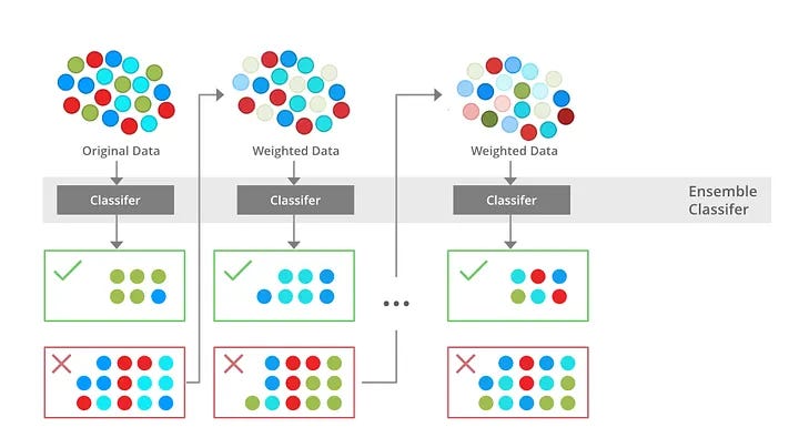
The process starts with a simple baseline prediction for every house. A common choice is the average price in the training data. This first prediction will not be accurate, but it gives the model a starting point. The important idea is that gradient boosting improves this starting point through many small steps.
Once we have the baseline predictions, we measure how far they are from the true prices. These differences are called residuals. If the model predicts 300 thousand but the house actually costs 350 thousand, the residual is 50 thousand. The next step is to train a small decision tree that tries to predict these residuals. This tree learns patterns in the errors, such as noticing that large houses in a certain neighborhood are consistently underpriced by the baseline model.
After training this tree, we add its predictions to the original baseline. This gives us slightly better predictions. Now the model makes new errors, and we repeat the process. Each new tree focuses on the mistakes still left over. Over many rounds the model becomes more accurate because it keeps learning what the earlier trees failed to capture.
The reason this method is called gradient boosting is because it uses gradients of the loss function to decide what each new tree should learn. The loss function tells us how bad the current predictions are. The gradient tells us the direction in which we need to adjust the predictions to reduce that loss. In a linear model, the gradient would update numeric weights. In gradient boosting, the gradient becomes the target for the next tree to fit. So each tree is essentially modeling the gradient of the loss with respect to the current predictions.
This gives gradient boosting two advantages. First, it can be used with many different loss functions, such as squared error for regression or logistic loss for classification. Second, it makes the updates smooth and controlled. Instead of making large jumps, the model adds small corrections at each step.
A second control mechanism is the learning rate. When we add the predictions from each tree, we usually scale them down. This prevents the model from taking corrections that are too large and helps reduce overfitting. It is similar to adjusting the seasoning in a dish slowly instead of making drastic changes after one tasting.
After many rounds, the final model is the sum of all these small trees. Each tree captures a different part of the pattern in the data. Together, they form a strong model that can represent complex relationships, like how houses in one area may follow different pricing rules than similar houses in another area.
This step by step improvement is the core of gradient boosting. XGBoost builds on this basic idea but makes the process faster, more stable and more accurate through better optimization and smarter system design.
The Training Process Step by Step
To understand how XGBoost learns, it helps to follow how each new tree adjusts the model’s predictions. Using the house price example, imagine the model already made an initial guess and now needs to improve it. XGBoost guides this improvement using a combination of derivatives, clever split evaluation, and regularization.
The entire process is anchored by the objective function. It combines the loss, which measures how far the predicted house prices are from the true values, with a penalty for building overly complex trees. Every update aims to reduce this objective, not only the training error. This is why XGBoost tends to build simpler, more generalizable models than plain gradient boosting.
To figure out how to reduce the objective, XGBoost does not directly look at the raw errors. Instead, it computes two values for each training example: the gradient and the hessian. For our house prices, the gradient tells XGBoost whether the prediction should move up or down. The hessian indicates how steep or confident the loss function is in that direction. These values act like compact signals summarizing how the model is performing at each point.
For squared error, the gradient is simply prediction minus actual price, so underpredicted houses have negative gradients and overpredicted houses have positive ones. The hessian is constant, which means the loss curve is simple. For other losses, especially in classification, the hessian provides extra information about the curvature of the loss and makes updates more precise.
Once the gradients and hessians are known, XGBoost begins examining potential splits in the next decision tree. For any candidate split, it looks at the examples that would go to the left and the right side, and it sums up their gradients and hessians. These sums, often written as G and G, capture the collective direction and confidence of errors in that region of the feature space. If one side contains many underpredicted houses, its G will be strongly negative. If another side contains mixed errors, its G may be small. This approach allows XGBoost to evaluate splits efficiently without revisiting raw labels. The beauty of this approach is that XGBoost does not need the original labels at this point. The derivatives alone carry enough information to evaluate splits.
From these aggregated values, XGBoost computes the optimal leaf score. This is the correction the model will add to predictions for any house landing in that leaf. The formula is simple and comes directly from optimizing the regularized objective:
Here G and H are sums of gradients and hessians for the leaf, and λ controls how strongly large leaf weights are penalized. If a leaf contains many houses that the model underpredicted by roughly 40 thousand, then G will be large and negative. The negative sign flips the direction, producing a positive correction to raise the predictions. The denominator ensures that the correction does not become too aggressive.
But before deciding that a split is worthwhile, XGBoost checks whether splitting the parent node actually improves the objective. It does this using the gain calculation. Gain compares how much the two new leaves would improve the objective versus leaving the node as one leaf:
A positive gain means the split produces a meaningful improvement by grouping houses with similar pricing errors. A negative or small gain means the split mostly captures noise. The term γ subtracts a small cost for creating a new leaf, ensuring that only useful splits are chosen.
These formulas together explain why XGBoost is so efficient. Everything the tree needs i.e. leaf scores, split quality, and corrections, is determined using only gradient and hessian sums. There is no need for repeated scans over the original labels.
As the tree grows, XGBoost always splits the leaf with the highest gain. This leaf-wise strategy allows the model to spend more depth where the patterns in house prices are richer and keep other branches shallow. It makes the model expressive but also increases the importance of regularization (controlled by γ and λ)
Even after computing the leaf score, XGBoost applies it cautiously. It multiplies the score by a learning rate, which slows down updates. If a leaf suggests increasing predictions by 40 thousand, a learning rate of 0.1 would apply only 4 thousand at that step. Later trees refine the value. This gradual adjustment helps the model remain stable and avoid overfitting.
When you put these pieces together, the training loop becomes easier to see.
Gradients and hessians identify errors.
Leaf scores compute the best corrections.
The gain calculation decides whether a split is worth it.
Leaf-wise growth focuses the model where improvement matters most.
And the learning rate ensures the model improves steadily rather than abruptly.
By repeating these steps tree by tree, XGBoost builds a model that captures complex patterns in house prices in a controlled, mathematically grounded way.
What Makes XGBoost Special
Once you understand how a gradient boosting model grows trees step by step, the natural question is why XGBoost performs so much better than older boosting methods. XGBoost became popular because it does several practical things extremely well. These are not small tweaks. They solve real problems that appear in messy, large, real-world datasets. Here are the ideas that make XGBoost stand out.
Regularization
The first important improvement is the way XGBoost uses regularization. In simple gradient boosting, the model tries to reduce the training error without paying much attention to tree complexity. This can lead to trees that are large, noisy or unstable. XGBoost fixes this by adding both L1 and L2 penalties directly into the objective function. L2 penalty shrinks leaf weights so that corrections are smaller and smoother. L1 penalty pushes very small leaf weights to exactly zero, which helps create simpler trees. Consider our house price example. If the model finds a tiny correction for a leaf containing only a few houses, L1 regularization may push that correction to zero, essentially saying, “This adjustment is not important enough.” This keeps the model focused on the most meaningful patterns.
Identifying Split Points
Another important improvement is how XGBoost finds good split points for each feature. In many datasets, a feature can have thousands of unique values. Traditional gradient boosting would check every possible value to decide where to split, which quickly becomes too slow. XGBoost solves this with a method called the weighted quantile sketch.
The key idea is that XGBoost does not need to test every possible value. Instead, it needs a small number of representative values that capture the shape of the feature and the importance of the samples. The sketch does this by summarizing the feature distribution while giving more influence to samples that have larger gradients and hessians. A sample with a large gradient is one the model is currently getting very wrong, so its value should matter more when choosing a split. The weighted sketch keeps track of these important samples without storing everything exactly.
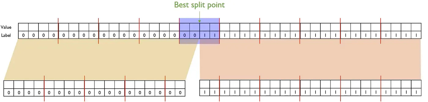
To understand how it helps, imagine the square footage feature in our housing dataset. Suppose it has many unique values, from small apartments to very large houses. XGBoost builds a sketch that approximates the distribution of square footage while incorporating the gradient and hessian of each house. Houses with larger errors effectively get more weight in the summary. The sketch then produces a set of candidate split points that represent important regions of the feature space. These might be boundaries between small, medium, and large homes, or regions where the model currently struggles the most.
During split finding, XGBoost evaluates only these candidate points, not every distinct value. This dramatically reduces the number of computations. Yet the splits remain effective because the sketch preserves the essential structure of the data, especially the parts where the model needs improvement.
The benefit is that XGBoost can process large datasets with many unique feature values while still choosing high quality splits. The weighted quantile sketch gives the model a smart, compact view of the feature distribution, saving time without sacrificing prediction accuracy.
Handling Missing Values
XGBoost also handles missing values intelligently. Many real datasets contain missing information, such as unknown lot size for a house. Instead of requiring manual imputation, XGBoost learns a default direction for missing values for each split. During training, the model tries sending all missing values to the left child and computes the objective, then sends them to the right child and computes it again. The direction that reduces the objective more becomes the learned default. During prediction, if a value is missing, it simply follows the learned direction. This allows the model to adapt to the structure of the data. For example, if missing square footage tends to occur in older or smaller homes, the model will discover that going to the smaller-home branch reduces error more, so it chooses that path automatically.
Parallel Training
To make training fast, XGBoost is designed to work in parallel. When building a tree, different features can be evaluated at the same time across CPU cores. In the house price example, one core may examine splits on number of rooms while another evaluates splits on house age. This is why XGBoost often trains much faster than older implementations of gradient boosting. On very large datasets, XGBoost can even distribute training across multiple machines.
Optimized Storage with DMatrix
XGBoost also introduces a special way to store data called DMatrix. Instead of storing your dataset as a regular table, DMatrix stores features in a compressed, column-based format. It also keeps track of which values are missing and provides fast access to the gradient and hessian for each example. This structure is optimized specifically for tree building. As a result, XGBoost uses less memory and looks up split information more efficiently, especially when dealing with large or sparse datasets.
When you put these pieces together, you can see why XGBoost became the go-to method for structured data. It is not just the boosting idea itself. It is the combination of regularization that stabilizes trees, faster split finding that scales to large data, intelligent handling of missing values, parallel computation and memory-efficient data structures. All these features work behind the scenes to make XGBoost both accurate and practical in everyday machine learning tasks.
Important Parameters and What They Control
Although XGBoost exposes many parameters, most of them influence only a few core behaviors: how complex the trees can become, how much randomness is introduced, how strongly leaf weights are regularized, how quickly the model learns, and how it handles imbalanced datasets. Understanding these groups is more useful than memorizing every single parameter. Once you see how each group shapes model behavior, tuning XGBoost becomes much more intuitive.
A major group of parameters governs tree complexity. The most noticeable one is max_depth, which controls how deep each tree is allowed to grow. Large values of max_depth give the model the freedom to learn detailed and specific patterns. In a house price dataset, this might allow the model to distinguish between subtle differences in property types or neighborhood characteristics. However, deep trees often memorize noise and overfit. Small values of max_depth restrict the tree to broader patterns and produce a more stable model, although they may underfit if the real relationships are complex. Another important parameter is min_child_weight, which sets the minimum sum of hessians required to create a new leaf. A large value makes the model cautious, allowing splits only when there is enough evidence. Small values permit the model to create leaves from smaller or noisier groups, increasing flexibility but also increasing the risk of learning patterns that do not generalize well. The gamma parameter also affects this behavior by requiring a minimum loss reduction before a split is made. With a large gamma, the model forms only splits that lead to clear improvement. With small gamma, XGBoost explores more detailed branches. In some tree methods, max_leaves additionally controls the maximum number of leaves, providing a direct limit on tree size.
A second group of parameters controls subsampling, which introduces helpful randomness. The subsample parameter specifies the fraction of training rows used to build each tree. If subsample is close to one, each tree uses almost the entire dataset, making the model more deterministic and sometimes prone to overfitting. Smaller values reduce variance by ensuring each tree sees a slightly different view of the data. Similarly, colsample_bytree, colsample_bylevel, and colsample_bynode determine the fraction of features used at different stages. When these values are small, each tree builds using different subsets of features, preventing the model from depending too heavily on any single predictor. When these values are large, the model has full access to all features, which can increase predictive power but may also capture noise.
Regularization parameters directly influence how leaf weights are adjusted. The lambda parameter applies L2 regularization, shrinking leaf weights toward zero. Large values of lambda make corrections smaller and more stable, while small values allow larger adjustments. The alpha parameter applies L1 regularization. When alpha is large, weak or noisy leaf weights are pushed to zero entirely, simplifying the tree by removing small contributions that do not strongly reduce the loss. When alpha is small, the model retains even minor adjustments. Another stability-related parameter is max_delta_step, which limits how much a leaf weight can change during one update. When set to a small value, this can stabilize training in tasks such as classification where gradients may be large.
One of the most influential parameters is the learning rate, called eta. This parameter scales the corrections made by each tree. When eta is small, each tree contributes only a slight adjustment, so the model learns slowly but safely. This usually improves generalization because the model moves through the loss landscape carefully instead of making abrupt jumps. When eta is large, each tree makes a stronger correction. This speeds up training but can cause the model to overfit early or miss better solutions. Most high performing XGBoost models use a smaller learning rate combined with a larger number of boosting rounds.
Training control parameters also play an important role. The n_estimators parameter specifies the number of boosting rounds. Too few rounds limit model capacity, while too many can cause overfitting unless early stopping is used. The early_stopping_rounds parameter monitors performance on a validation set and stops training when improvement stalls. This ensures training ends when the model has learned all the useful information without drifting into overfitting.
Finally, XGBoost includes parameters for handling imbalanced data. The scale_pos_weight parameter increases the importance of the positive class during training. If the positive class is rare, as in predicting rare property types or unusual sale outcomes, a larger scale_pos_weight makes the model pay more attention to these examples. Small or default values treat both classes equally, which can cause the model to ignore the minority class. In combination with this, max_delta_step sometimes helps stabilize updates when positive examples are scarce.
These parameters influence how trees grow, how much variation the model sees during training, how strongly it regularizes leaf weights, how quickly it learns, and how it handles skewed data. Once you understand how large or small values change the model’s behavior, tuning XGBoost becomes a process of shaping its capacity and stability rather than guessing settings.
Feature Importance in XGBoost
After training an XGBoost model, one of the first things people look at is feature importance. It helps you understand which features the model relied on most when making predictions. XGBoost provides several ways to measure importance, and each method captures a slightly different perspective of how the model used a feature. The three common types are weight, gain and cover. Understanding how they work, when they differ and what pitfalls to avoid makes you much more confident when interpreting an XGBoost model.
The simplest measure is weight. This counts how many times a feature was used in splits across all the trees in the model. If a feature appears in many splits, its weight is high. This measure is easy to understand, but it can be misleading. For example, a feature might appear often in shallow splits that do not reduce the loss very much, yet its weight would still be high. Another feature might appear only a few times but at very important points in the tree, and weight would not capture its influence.
Gain is usually the most meaningful measure. It represents how much a feature contributed to reducing the loss when it was used in a split. Every time XGBoost splits on a feature, it calculates a gain from that split. The total gain for a feature is the sum of these improvements. Features with high gain helped the model make more accurate predictions. In practice, gain often highlights the truly impactful features, since it reflects actual error reduction rather than just split frequency.
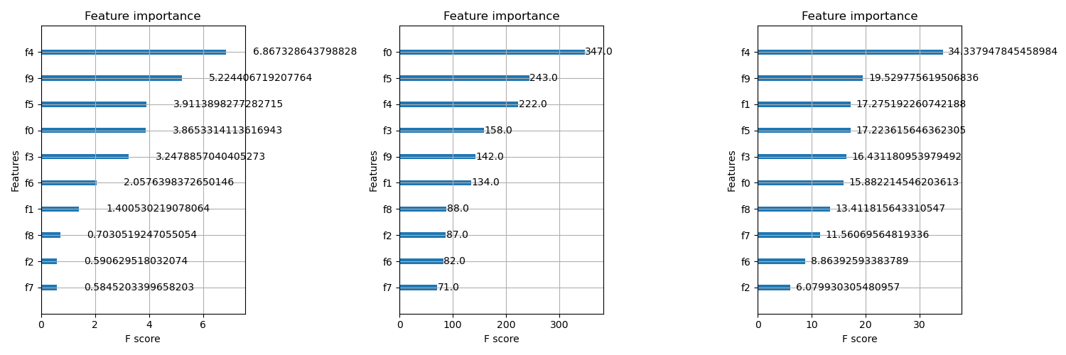
Cover measures how many samples are affected by splits that use a feature. If a feature is used in a split that affects many rows of data, its cover value increases. This may reveal features that consistently influence large portions of the dataset, even if the gain from each split is modest. For example, a feature like square footage in the housing dataset might appear early in the tree, splitting a large number of houses. Its cover would be high even if the gain per split is not the highest.
These three metrics often differ because they capture different aspects of the model’s behavior. A feature might have high weight but low gain if it appears often but does not make strong improvements. Another feature might have high gain but low cover if it produces significant improvement for a small group of samples. Features that have high cover but moderate gain may be broadly useful but not particularly decisive. Understanding these differences helps you interpret the model more accurately rather than relying on a single metric.
There are also some pitfalls to keep in mind. Feature importance values in tree models are not causal. A high importance score means the model relied on that feature, not that the feature directly caused the outcome. Correlated features can also distort importance scores. If two features carry similar information, the model may choose one and ignore the other, making the second appear unimportant even though it contains useful information. Another limitation is that importance scores do not reveal directionality. You cannot tell whether increasing a feature increases or decreases the prediction simply by looking at importance. Finally, importance scores depend on the training data distribution. If the dataset changes, the importance rankings may shift as well.
A few best practices help avoid misinterpretation. It is often useful to compare different importance metrics together rather than relying on one. If possible, inspect importance across cross validation folds to see whether patterns are consistent. For high stakes decisions, consider complementing tree based importance with methods like SHAP values, which provide more detailed explanations. And always remember that importance scores describe model behavior, not real world relationships.
Feature importance in XGBoost is a powerful tool for understanding your model, but it is most useful when interpreted carefully. By knowing what weight, gain and cover measure and where they differ, you can extract insight without falling into common traps.
Practical Optimization and Tuning in XGBoost
Once you understand how XGBoost builds trees and why it performs well, the next step is learning how to train models efficiently and avoid common issues such as overfitting or slow training. XGBoost provides many tools for this, and they fall into three broad categories: practical optimization techniques, system level improvements and hyperparameter tuning strategies. Together, these ideas help you build models that are accurate, efficient and well suited for real datasets.
A common challenge when training XGBoost is preventing overfitting. Because the algorithm can learn very detailed patterns, it may start fitting noise if the trees grow too large or if the model continues training long after it has extracted the important structure. Several techniques help reduce this risk. Limiting tree complexity through parameters such as max depth, min child weight and gamma prevents the model from creating overly specific branches. Subsampling rows and columns introduces randomness into training and encourages the model to learn broader patterns rather than memorizing individual examples. Regularization through lambda and alpha keeps leaf weights small and stable. Finally, early stopping is a practical safety mechanism. By monitoring performance on a validation set and stopping when improvements stall, you avoid adding trees that only reduce training loss but do not generalize.
Training speed is another practical concern, especially for large datasets. Several strategies help improve performance. Reducing max depth and using subsampling values below one shorten training time because each tree covers fewer rows and fewer features. Choosing a suitable tree method, such as the histogram based method, speeds up split finding by grouping feature values into bins. Setting a reasonable learning rate and limiting the number of boosting rounds avoids unnecessary computation. Even small adjustments to these parameters can make training significantly faster without hurting performance.
Memory efficiency matters when working with large or sparse datasets. XGBoost’s DMatrix format is designed specifically for this. It stores the data in a compact, column oriented format that allows quick access to each feature. It also records missing and zero values efficiently, which is important because many real datasets, especially in domains like text or retail, contain sparse features. Using the histogram tree method can also reduce memory usage because it works with binned values instead of storing individual numbers.
Choosing the right evaluation metric is another practical element of training. XGBoost supports metrics such as RMSE for regression, log loss or error for classification and AUC for ranking tasks. The choice depends on your goal. For example, predicting house prices usually uses RMSE because it penalizes larger errors more, while classification tasks often use log loss when you care about calibrated probabilities. Selecting the correct metric ensures you optimize the model for the outcome that matters most.
Beyond these high level techniques, XGBoost includes system level optimizations that make training faster and more scalable. Parallel split finding is one of the most important. When evaluating splits, XGBoost can compute histogram statistics for many features at the same time across multiple CPU cores. Instead of scanning features one by one, it processes them in parallel, reducing the time needed to build each tree. This is especially useful when training many models during tuning. Another system level capability is out of core training, which helps when the dataset does not fit into memory. XGBoost can read data in batches from disk, process the gradients and hessians and accumulate them efficiently. This allows training on datasets far larger than RAM would allow. Sparse data handling is also built into the design. XGBoost automatically skips over missing and zero values when computing histograms and learns default directions for missing values during split finding. This avoids the cost of manual imputation and often leads to better results.
Once you have an understanding of how XGBoost behaves, hyperparameter tuning becomes the next step. There are several common strategies. Grid search tries all combinations of chosen parameter values and is simple to set up, although it becomes expensive when the search space is large. Random search samples random combinations from a parameter distribution. This often finds good configurations faster because not all parameters influence performance equally. Bayesian optimization takes the process further by using past trial results to choose the next promising parameter combination. It balances exploration and exploitation, usually finding strong models with fewer evaluations.
Regardless of the search method, a practical tuning workflow usually begins by controlling the overall complexity of the model. You often start by selecting a reasonable max depth and min child weight that prevent clear overfitting. Next, you choose appropriate subsampling values to add randomness and improve generalization. After that, you tune regularization parameters such as lambda and alpha to stabilize the model further. Only after these structural and regularization parameters are set does it make sense to fine tune the learning rate and number of trees, often with early stopping support. This structured approach helps you avoid wasting time on learning rate adjustments when the underlying tree settings are already causing overfitting.
Bringing these ideas together gives you a solid foundation for training efficient and accurate XGBoost models. Practical optimization techniques guide how to avoid overfitting and how to train quickly. System level optimizations ensure your model can scale to large datasets. Tuning strategies help you search the parameter space effectively. Once you combine these ideas, XGBoost becomes not only a powerful algorithm but also a practical tool for real machine learning projects.
Common Interview Questions and How to Answer
Interviewers frequently ask about XGBoost because it combines algorithmic ideas, practical engineering and real world behavior. Strong answers show that you understand both the mathematics and how the model behaves in practice. Below are 15 common questions with concise, technically accurate answers.
1. What problem does XGBoost solve compared to standard Gradient Boosting?
XGBoost improves gradient boosting through regularization, second order optimization, efficient split finding, built in handling of missing values, and extensive system level optimization. It is designed for speed, scalability and robustness, making it more effective on large or messy datasets.
2. Why does XGBoost use second order gradients instead of only first order gradients?
Second order gradients provide curvature information. The hessian helps the model judge how confident it should be in the gradient direction. This allows closed form leaf weight calculations, more stable updates and better optimization, especially in classification tasks.
3. How does XGBoost compute the leaf score?
Leaf scores minimize a regularized second order Taylor expansion of the loss. The optimal score is w∗=−G/(H+λ). This uses the sum of gradients and hessians to decide how much to adjust predictions in that region.
4. What is the gain formula and what does it represent?
Gain measures how much the objective improves when a node is split into two. It compares the improvement from the children to the improvement from the parent and subtracts a penalty. The split with the highest gain is chosen. Gain connects directly to error reduction.
5. How does XGBoost handle missing values?
During split finding, XGBoost evaluates whether sending missing values to the left or right child yields a lower objective. It learns a default direction for missing values, which is then used during prediction. This avoids manual imputation and often improves accuracy.
6. What is the weighted quantile sketch and why is it used?
It is an algorithm that approximates quantiles of feature values while weighting samples by their gradient and hessian. This allows XGBoost to pick a small number of promising split points efficiently instead of checking every unique feature value.
7. What happens when two features are highly correlated?
XGBoost typically picks one feature for splits and ignores the other. This reduces the apparent importance of the second feature. It does not create instability, but it does mean feature importance should be interpreted cautiously when correlation is high.
8. How does subsampling rows and columns help?
Row subsampling forces each tree to train on slightly different subsets, reducing variance and overfitting. Column subsampling prevents the model from over relying on a small group of strong features. Both also speed up training.
9. When should you use a small learning rate in XGBoost?
A small learning rate improves generalization by applying corrections slowly and allowing later trees to refine the prediction. It is useful when you can afford more boosting rounds and want a stable model with reduced overfitting.
10. What is the effect of increasing max_depth?
A larger max_depth allows the model to capture complex interactions but increases the risk of overfitting. In practice, values between 3 and 10 work well. Deep trees should be balanced with strong regularization or subsampling.
11. How do you handle imbalanced classification with XGBoost?
Set scale_pos_weight to the ratio of negative to positive samples, adjust max_delta_step for stability if needed, and consider using evaluation metrics such as AUC or F1. This forces the model to give more weight to the minority class.
12. Why is regularization important in XGBoost?
Regularization terms lambda and alpha shrink or zero out leaf weights. This prevents trees from making overly aggressive corrections and reduces overfitting. It is one of the main reasons XGBoost performs better than plain gradient boosting.
13. What tree method should you use for large datasets?
The histogram based tree method is usually best. It bins feature values, reduces memory usage and speeds up split finding dramatically. It is the default in many implementations for scalable training.
14. How do you tune XGBoost effectively?
Start by tuning tree complexity (max_depth, min_child_weight), then subsampling parameters (subsample, colsample_bytree), then regularization (lambda, alpha). After stabilizing the model, tune learning rate and number of estimators with early stopping. Use random search or Bayesian optimization for efficiency.
15. Why does XGBoost often outperform Random Forests?
XGBoost reduces residual errors step by step, optimizes splits using gradients and hessians, and applies regularization. Random forests average many independent trees, while XGBoost builds trees sequentially based on error patterns. This often gives XGBoost higher accuracy on structured data.
Summary and Final Tips
XGBoost can feel complex at first, but once you understand the ideas behind boosting, the algorithm becomes much more intuitive. Boosting is the process of improving a weak model step by step by learning from the mistakes made so far. Each tree does not need to be powerful on its own. Instead, the strength comes from the sequence of small, targeted corrections. XGBoost enhances this idea with second order optimization, regularization and efficient engineering. When you think about boosting this way, it becomes easier to explain its behavior and answer interview questions confidently.
Before interviews, it helps to focus on a few core concepts. Make sure you understand how gradients and hessians are used, how leaf scores and gains are calculated and why regularization is built into the objective. Be able to describe split finding, missing value handling and the weighted quantile sketch in simple language. It is also useful to remember how parameters influence the model. Interviewers often ask what happens when you increase max depth or lower the learning rate, not because they care about exact numbers but because they want to see if you understand model behavior. Finally, be ready to compare XGBoost with random forests or basic gradient boosting and explain what makes XGBoost more stable and more scalable.
With these ideas in mind, you should be well prepared for XGBoost questions in interviews. More importantly, you will have a deeper understanding of how boosting works and how to use it effectively in real projects.
Wow! Very nice and just in time. Great reminder, liked how you walk through all steps from helicopter view to steps of implementation.