
Data Science Interview Guide - Part 3: Logistic Regression
Understanding log-odds, practical tips to fit log reg, and common interview questions

If you’ve ever sat in a data science interview, chances are you’ve been asked about Logistic Regression. Despite being one of the oldest algorithms in the machine learning toolkit, it continues to be one of the most important — and one of the most misunderstood.
At first glance, Logistic Regression might look like a close cousin of Linear Regression — and in many ways, it is. But while Linear Regression predicts continuous values, Logistic Regression predicts probabilities, helping us decide whether an email is spam, a transaction is fraudulent, or a customer is likely to churn. This simple switch — from predicting numbers to predicting probabilities — makes Logistic Regression the gateway to understanding classification, one of the core pillars of machine learning.
In data science, Logistic Regression holds a special place because it’s both interpretable and powerful. It offers clear mathematical intuition while still being practical enough to deploy in real-world systems. That balance of simplicity and explainability makes it a favorite for interviews — hiring managers want to see if you truly understand the foundation before diving into complex models like XGBoost or neural networks.
This blog is your crash course to master Logistic Regression from an interview perspective — we’ll explore its assumptions, how it’s optimized, how to evaluate it, and the kinds of questions interviewers love to ask.
By the end, you won’t just know the math — you’ll know how to talk about it like a pro.
What is Logistic Regression?
At its core, Logistic Regression is a classification algorithm used to predict discrete outcomes — most commonly, a binary one:
Will a customer churn or stay?
Is this transaction fraudulent or legitimate?
Does this image contain a cat or not?
While the name includes regression, the goal isn’t to predict continuous numbers but rather probabilities. Logistic Regression estimates the likelihood that an observation belongs to a certain class — typically labeled as 0 or 1.
So how does it work?
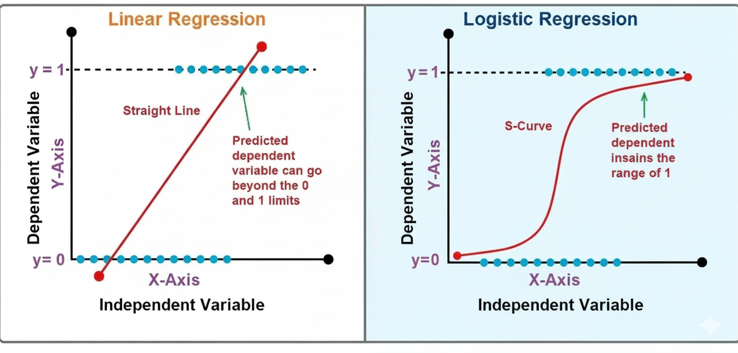
Imagine fitting a straight line, like in Linear Regression, but instead of directly predicting outputs like 10, 20, or 30, we want outputs between 0 and 1 — values that can represent probabilities. To achieve this, Logistic Regression applies the sigmoid function to the linear equation:
This squashes any real-valued number into a range between 0 and 1. When p is greater than 0.5, we classify the outcome as 1; otherwise, it’s 0.
The model’s coefficients βi determine how each feature influences the log-odds of the outcome. Unlike Linear Regression, where coefficients affect the mean of the target, here they affect how the odds tilt toward one class or the other.
Mathematically elegant, computationally efficient, and intuitively clear — Logistic Regression is often the first stop in the journey from regression to classification.
It’s simple enough to be explainable, yet powerful enough to serve as the foundation for many advanced models in machine learning, from neural networks to credit risk scoring systems.
What is Logistic Regression?
At first glance, Logistic Regression sounds like a strange name for something used in classification. After all, “regression” usually refers to predicting numbers, not categories.
But Logistic Regression isn’t really about regression in the everyday sense — it’s about modeling probabilities that something belongs to one class or another.
Let’s start simple.
From Linear Regression to Classification
Linear Regression fits a straight line through data to predict continuous outcomes like house prices or sales numbers. Mathematically, it looks like this:
The output yyy can take any value — from negative infinity to positive infinity.
But what if we’re not trying to predict a continuous value?
What if we want to predict whether something is yes or no, spam or not spam, disease or no disease?
That’s where Linear Regression fails — because probabilities must always lie between 0 and 1, while a straight line can easily predict values outside that range.
Enter Logistic Regression
Logistic Regression fixes this by transforming the linear output into a probability using a special function called the sigmoid (or logistic) function.
The sigmoid function takes any real number and “squeezes” it into a value between 0 and 1:
Here:
p represents the probability of the positive class (for example, “1” = spam, churn, fraud, etc.).
1−p represents the probability of the negative class (“0”).
The coefficients βi determine how strongly each feature influences that probability.
Once we have the probability p, we can easily classify outcomes:
If p>0.5, predict 1
If p≤0.5, predict 0
This simple threshold converts a smooth probability curve into a crisp decision boundary.
Understanding the Log-Odds (The “Logit”)
The term Logistic Regression actually comes from modeling the log-odds (also known as the logit) of the probability.
Odds represent how much more likely an event is to happen than not to happen:
Odds=p/(1−p)
Taking the logarithm gives us the log-odds:
This relationship is linear in the coefficients — meaning we can still use many of the same tools as in linear regression (like gradient-based optimization).
That’s the beauty of Logistic Regression: it connects linear relationships with probabilistic reasoning.
Why It Matters
Logistic Regression is often the first classification model every data scientist learns — and for good reason:
It’s mathematically interpretable — you can explain exactly how each feature affects the odds of an outcome.
It’s computationally efficient, even on large datasets.
It provides probability estimates, not just hard labels.
And it forms the foundation for more advanced models like neural networks and generalized linear models (GLMs).
Despite being conceptually simple, Logistic Regression is still widely used in production systems — from credit scoring and medical diagnosis to recommendation systems and customer churn prediction.
In short, Logistic Regression is where statistics meets machine learning — and understanding it deeply will give you intuition that carries into every other classification algorithm you’ll learn.
Assumptions of Logistic Regression
Like every statistical model, Logistic Regression rests on a few key assumptions.
These aren’t just theoretical details — understanding them helps you diagnose problems, justify modeling choices, and explain trade-offs in interviews and real-world projects. Let’s unpack them one by one.
The Dependent Variable is Binary (or Categorical)
Logistic Regression is designed for classification problems — typically binary ones.
That means your target variable should represent two possible outcomes:
1 = Event happens (e.g., customer churns, email is spam)
0 = Event does not happen
When you have more than two categories, you can use extensions like Multinomial Logistic Regression (for multiple classes) or Ordinal Logistic Regression (for ordered categories).
Interview insight:
You can confidently explain that Logistic Regression models the probability of a binary outcome using a logistic function — not the outcome itself.
Independence of Observations
Each observation in your dataset should be independent of others.
For example, if you’re predicting whether users will buy a product, each user should be treated as a separate, unrelated case.
If the data points are correlated — say, multiple transactions from the same customer or repeated measures from the same patient — the model’s standard errors and significance tests become unreliable.
In such cases, we often turn to Generalized Estimating Equations (GEE) or Mixed-Effects Logistic Regression, which account for correlated data.
Think of it like this: Logistic Regression assumes each data point tells a unique part of the story — not the same story twice.
Linearity Between Features and Log-Odds
This is one of the most misunderstood assumptions.
Logistic Regression doesn’t assume a linear relationship between predictors and the target variable itself.
Instead, it assumes a linear relationship between the independent variables and the log-odds of the dependent variable.
In equation form:
That means each feature’s contribution is additive in the log-odds space, not directly in probability space.
If this linearity assumption is violated, the model can misrepresent relationships, leading to biased predictions.
Pro tip: Use transformations (like log or polynomial terms) or non-linear models to handle non-linear relationships.
No (or Minimal) Multicollinearity
Multicollinearity occurs when independent variables are highly correlated with each other.
This makes it difficult for the model to determine the unique effect of each variable — inflating variance in coefficient estimates.
You can detect multicollinearity using:
Variance Inflation Factor (VIF) — values above 5 (or 10) suggest trouble.
Correlation matrices — to identify redundant features.
To fix it, you can remove correlated variables, use Principal Component Analysis (PCA), or apply regularization (like Ridge or Lasso Logistic Regression).
Interview angle: If asked about dealing with multicollinearity, mention using VIF or L2 regularization to stabilize coefficient estimates.
Sufficiently Large Sample Size
Logistic Regression relies on Maximum Likelihood Estimation (MLE) to find the best-fitting coefficients.
MLE performs better with larger sample sizes — because it needs enough data to estimate probabilities accurately, especially for the minority class.
A rough guideline:
You should have at least 10–15 observations per predictor variable, ideally with a balanced number of positive and negative outcomes.
In small-sample situations, consider using penalized Logistic Regression or Bayesian methods for more stable estimates.
Absence of Outliers with Undue Influence
Outliers can disproportionately affect the fitted coefficients since the model tries to fit all points as best as possible.
Use diagnostic tools like - Cook’s Distance, Leverage values, Standardized residuals to detect and manage influential points.
While these assumptions might sound restrictive, they’re often manageable in practice. Understanding them gives you a mental framework for why Logistic Regression behaves the way it does, and more importantly — helps you explain when it might fail.
How Logistic Regression is Optimized
Once we know what Logistic Regression does — predicting probabilities for categorical outcomes — the next question is:
How does it actually learn those probabilities?
Linear Regression finds the best-fit line by minimizing the sum of squared errors.
But Logistic Regression doesn’t predict continuous numbers — it predicts probabilities using a sigmoid function, which is nonlinear.
So, the same least-squares trick won’t work here.
Instead, Logistic Regression relies on a powerful idea from statistics called Maximum Likelihood Estimation (MLE) — it learns the parameters that make the observed data most probable under the model.
From Probabilities to Likelihood
For each data point iii, the model predicts the probability of the positive class as:
Here:
pi = predicted probability that yi=1y_i = 1yi=1
xij = value of feature jjj for sample iii
βj = weight (coefficient) the model is trying to learn
Now, depending on whether the true label yiy_iyi is 0 or 1, the probability of observing that label is:
If yi=1, the probability is pi.
If yi=0, the probability is 1−pi.
So this formula elegantly handles both cases in one expression.
For all m observations, we multiply these probabilities together (assuming independence) to get the likelihood:
This is the probability of the entire dataset given the parameters β. The goal is to find the coefficients that make this overall likelihood as large as possible.
The Log-Likelihood Function
Products of many small probabilities can quickly underflow to zero numerically, so we take the logarithm (which turns products into sums) to get the log-likelihood:
Each data point contributes to the overall score depending on how confident and correct the model was:
If the model correctly predicts a high pip_ipi for a positive sample, log(pi) is large → high reward.
If it predicts a low pip_ipi for a positive sample, log(pi) is very negative → strong penalty.
That’s why the model “learns” by maximizing this function — it’s literally rewarding correct confidence and punishing confident mistakes.
The optimization goal is:
Or equivalently (since maximization and minimization are mirror problems):
The negative log-likelihood is what’s commonly known as the Binary Cross-Entropy Loss or Log Loss:
Log Loss measures how uncertain or wrong the model is.
A perfect model has Log Loss = 0.
As predictions become uncertain (closer to 0.5), the penalty increases sharply — reflecting the cost of indecision.
Gradient Descent: The Learning Mechanism
Unlike Linear Regression, we can’t solve for β\betaβ directly because of the sigmoid’s nonlinearity.
So we use Gradient Descent, an iterative optimization algorithm.
At each step, we compute the gradient (the slope of the loss function with respect to each coefficient) and move in the opposite direction of that slope — the direction that reduces the loss.
Where:
α is the learning rate — how big each step is
∂J(β)/∂βj is the gradient — showing how sensitive the loss is to that coefficient
Think of it like hiking downhill in fog — you don’t see the whole mountain, but you can feel which direction slopes downward, and take small steps until you reach the valley (the minimum).
Over time, the model “descends” to the set of parameters that minimize the loss — i.e., maximize the likelihood.
Regularization: Avoiding Overfitting
When features are many or correlated, Logistic Regression can overfit — memorizing patterns that don’t generalize.
To fix that, we add regularization, a penalty term that discourages overly large coefficients.
L2 Regularization (Ridge)
Adds a squared penalty to the loss function:
Keeps coefficients small and smooth, distributing influence across many features.
L1 Regularization (Lasso)
Adds an absolute value penalty:
Pushes some coefficients exactly to zero — effectively performing feature selection.
The parameter λ controls how strong the penalty is. A higher λ means simpler models (less overfitting) but potentially less flexibility.
At a high level:
Logistic Regression tries to find parameters that maximize the likelihood of seeing your data.
The math turns that problem into minimizing Log Loss.
Gradient Descent adjusts parameters step by step to find the best fit.
Regularization keeps the model from memorizing noise.
It’s a dance between fitting the data well and staying humble enough to generalize.
Common Evaluation Metrics for Logistic Regression
Once your Logistic Regression model is trained, the next step is figuring out how well it performs.
Accuracy alone often paints a misleading picture — especially when your data is imbalanced (like fraud detection or medical diagnosis).
That’s why it’s essential to understand the key evaluation metrics that tell the true story of your model’s performance.
Let’s unpack the most important ones.
The Confusion Matrix
Every evaluation metric stems from one simple concept — the confusion matrix.
It compares the model’s predicted labels with the actual ones.
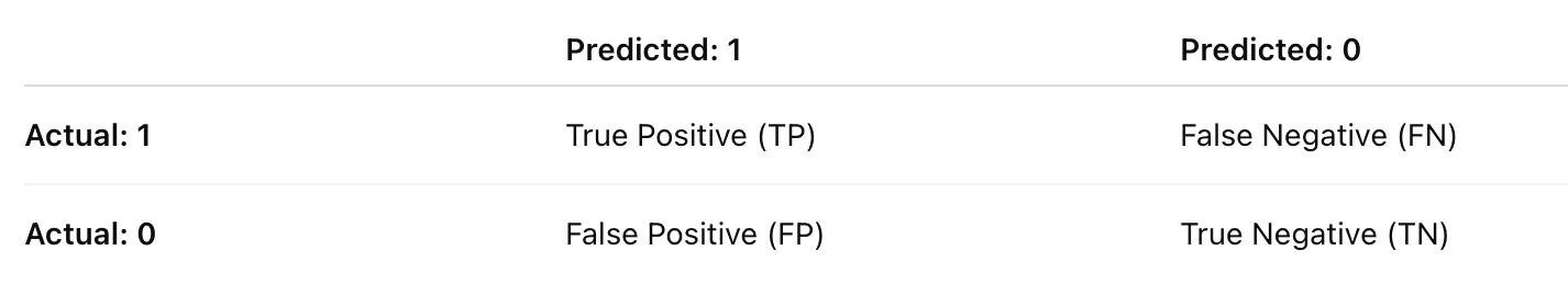
TP: Model correctly predicts the positive class
FP: Model incorrectly predicts positive
FN: Model misses a positive
TN: Model correctly predicts the negative
From this matrix, we derive all the other metrics.
Accuracy
Accuracy tells you how often the model was correct overall.
✅ Intuition:
Accuracy is great when both classes are equally important and balanced.
But if your dataset is 95% “No Fraud” and 5% “Fraud,” a model that always predicts “No Fraud” will still be 95% accurate — yet completely useless.
That’s why we need precision, recall, and F1.
Precision
Precision answers the question - Of all the positive predictions the model made, how many were actually correct?
High precision means the model rarely cries wolf — when it says “Positive,” it’s usually right. In fraud detection, high precision means you’re not falsely accusing legitimate transactions.
Recall (Sensitivity or True Positive Rate)
Recall measures how many of the actual positives the model managed to catch.
In other words - Out of all the fraudulent transactions, how many did the model detect?
High recall means fewer missed positives — but possibly more false alarms.
Precision and recall often trade off against each other.
Tuning your model to increase one usually lowers the other.
F1-Score: The Balance Between Precision and Recall
F1 is the harmonic mean of precision and recall.
It’s high only when both are high — making it a balanced metric for imbalanced datasets.
If you care equally about catching positives and avoiding false alarms, F1 is often the go-to metric.
Interview insight:
If asked “Why use the harmonic mean instead of the arithmetic mean?”, explain that the harmonic mean penalizes extreme imbalances — e.g., high precision but very low recall.
ROC Curve and AUC (Area Under Curve)
Logistic Regression produces probabilities, not just binary labels.
To decide whether a sample is 0 or 1, you pick a threshold — usually 0.5.
But you can vary this threshold to explore how sensitivity (recall) and specificity (1 – false positive rate) change.
The ROC curve (Receiver Operating Characteristic curve) plots:
X-axis: False Positive Rate (FPR)
Y-axis: True Positive Rate (TPR = Recall)
The AUC (Area Under Curve) summarizes this curve into a single number between 0 and 1.
AUC = 0.5 → model is guessing randomly.
AUC = 1.0 → perfect separation between classes.
AUC = 0.8 → on average, model ranks a random positive higher than a random negative 80% of the time.
AUC is particularly valuable when your data is imbalanced because it measures ranking quality — not just accuracy at one threshold.
Log Loss (Binary Cross-Entropy)
Finally, the metric most closely tied to how the model is trained:
Log Loss penalizes confidence in the wrong direction.
Predicting 0.9 for a positive case (correctly confident) is rewarded.
Predicting 0.9 for a negative case (confidently wrong) is heavily punished.
It encourages the model not only to be right but to be calibrated — meaning its predicted probabilities match real-world likelihoods.
Choosing the Right Metric
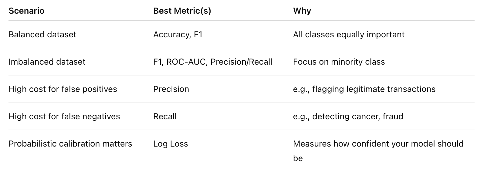
Each metric highlights a different aspect of model performance:
Accuracy tells you how often you’re right.
Precision tells you how trustworthy your positive predictions are.
Recall tells you how complete your detection is.
F1 balances those two.
AUC tells you how well your model separates classes overall.
Log Loss tells you how confident and calibrated your probabilities are.
In interviews, being able to choose the right metric — and justify why — is often the difference between a surface-level answer and one that shows deep practical understanding.
Practical Tips and Pitfalls
Logistic Regression may look simple, but in practice, it’s full of subtle traps.
Many models that appear “fine” on paper fail quietly because of poor preprocessing, untested assumptions, or misinterpreted coefficients.
Let’s look at the most important best practices and common pitfalls — and how to avoid them.
Always Scale or Normalize Continuous Features
Logistic Regression is sensitive to feature scales because it uses gradient-based optimization.
If one feature (say, “income”) ranges from 0–100,000 and another (say, “age”) ranges from 0–100, the large-scale feature will dominate the optimization steps.
✅ Best practice:
Standardize or normalize your features before training:
from sklearn.preprocessing import StandardScaler

scaler = StandardScaler()
X_scaled = scaler.fit_transform(X)
Scaling ensures the optimization landscape is smooth, allowing the gradient descent to converge efficiently without oscillations.
Handle Categorical Variables Properly
Logistic Regression works with numeric inputs, so categorical features (like city, department, or product type) must be encoded.
Common encoding methods:
One-Hot Encoding: for nominal categories (e.g., “Red”, “Green”, “Blue”)
Ordinal Encoding: for ordered categories (e.g., “Low”, “Medium”, “High”)
Pitfall to avoid:
Including all dummy variables without dropping one can cause perfect multicollinearity — known as the dummy variable trap.
pd.get_dummies(df[’color’], drop_first=True)
Interview insight:
You can mention that one-hot encoding preserves interpretability — each coefficient compares that category to the baseline category that was dropped.
Watch Out for Multicollinearity
Highly correlated predictors make it difficult for the model to estimate the unique effect of each variable — leading to unstable coefficients.
Detect it:
Use the Variance Inflation Factor (VIF):
from statsmodels.stats.outliers_influence import variance_inflation_factor

vif = [variance_inflation_factor(X.values, i) for i in range(X.shape[1])]
Fix it:
Drop redundant variables
Combine correlated features (e.g., take averages)
Use L2 regularization (Ridge) to shrink correlated coefficients smoothly
Rule of thumb: VIF > 5 (or 10) indicates serious multicollinearity.
Regularization Isn’t Optional
Without regularization, Logistic Regression can overfit, especially in high-dimensional data (many features, few samples).
Add a penalty to control model complexity:
L1 (Lasso) — useful for sparse models and feature selection
L2 (Ridge) — preferred when most features are relevant
Pro tip:
Start with Ridge (default in scikit-learn), then try Lasso if you suspect many irrelevant variables.
Be Careful with Imbalanced Data
In cases like fraud detection or rare disease prediction, the positive class might be <5% of all samples. A model that predicts “no fraud” every time could have 95% accuracy — but be completely useless.
Best practices:
Use stratified train-test splits so both sets preserve class balance
Evaluate using Precision, Recall, F1, or ROC-AUC, not just accuracy
Adjust class weights or decision thresholds
Try SMOTE (Synthetic Minority Oversampling Technique) to generate synthetic minority examples
from imblearn.over_sampling import SMOTE
smote = SMOTE()
X_res, y_res = smote.fit_resample(X, y)
Don’t Forget Feature Interaction
Logistic Regression assumes a linear relationship in the log-odds space.
If features interact (say, “income” and “education”), the model might miss it.
Add interaction terms manually or use polynomial features:
from sklearn.preprocessing import PolynomialFeatures

poly = PolynomialFeatures(interaction_only=True, include_bias=False)
X_interact = poly.fit_transform(X)
You’re explicitly telling the model: sometimes two variables together have a different effect than each one alone.
Check Model Calibration
A well-trained model should not just predict correctly but also assign realistic probabilities.
For example, when your model says “this transaction has a 70% chance of fraud,” that should roughly mean that 70% of such cases are indeed fraudulent.
Check calibration:
Plot predicted probabilities vs actual outcomes using a calibration curve.
Fix it if needed:
Use Platt scaling or isotonic regression to recalibrate.
from sklearn.calibration import CalibratedClassifierCV

calibrated_model = CalibratedClassifierCV(base_estimator=log_reg, method=’isotonic’)
calibrated_model.fit(X_train, y_train)
Monitor for Overfitting and Underfitting
Overfitting: Model performs well on training but poorly on validation.
→ Use regularization or collect more data.Underfitting: Model performs poorly everywhere.
→ Add interaction terms, try nonlinear transformations, or move beyond Logistic Regression.
Pro tip:
Plot learning curves — they tell you instantly whether you need more data or a simpler model.
Interpret Coefficients Carefully
Remember: Logistic Regression coefficients are in log-odds space.
To make them interpretable, exponentiate them:
An odds ratio of 1.5 means that for every 1-unit increase in xj, the odds of the positive class increase by 50%. But beware — this interpretation holds only when other variables are held constant.
Don’t Treat Logistic Regression as “Too Simple”
In interviews, it’s tempting to rush through Logistic Regression as “basic.”
But in reality, it’s the foundation of nearly every classification model — including neural networks, which use a sigmoid activation in their final layer.
Common Interview Questions on Logistic Regression
Logistic Regression is a favorite interview topic because it combines theory, math, and practical intuition — all in one elegant model.
Below are the most common questions you’ll encounter, along with the kind of answers that impress interviewers.
1. Why use Logistic Regression instead of Linear Regression for classification?
At first glance, it might seem that Linear Regression could do the job — just draw a line and assign class 1 for values above 0.5.
But there are two key problems:
Unbounded outputs:
Linear Regression can predict values below 0 or above 1 — which makes no sense for probabilities.Non-constant variance (heteroscedasticity):
The residuals won’t have constant variance because of the bounded nature of probabilities.
Logistic Regression fixes both by mapping linear outputs into probabilities using the sigmoid function:
Say that Logistic Regression ensures outputs are always between 0 and 1, and it models the log-odds linearly, which aligns with probability theory.
2. What does the coefficient in Logistic Regression represent?
Each coefficient βj represents the change in the log-odds of the outcome for a one-unit change in that predictor, holding others constant.
If β1=0.7, then increasing x1 by 1 increases the odds of the positive class by e^{0.7} ≈2.01 — about twice as likely. Interviewers love when candidates move smoothly from the coefficient → log-odds → odds → probability interpretation.
Looking to land your next role? The two hurdles you need to tackle are callbacks and interviews.
To get a callback, make sure your resume is well-written with our resume reviews, where we provide personalized feedback - https://topmate.io/buildmledu/1775929
To crack interviews, use our mock interview services. Whether it’s DSA, ML/Stat Theory, or Case Studies, we have you covered - https://topmate.io/buildmledu/1775928

Don’t forget, for everything ML - Checkout BuildML
https://topmate.io/buildmledu
3. Why do we use Maximum Likelihood Estimation (MLE) in Logistic Regression?
In Linear Regression, minimizing squared errors gives the best-fit line.
But Logistic Regression’s sigmoid function makes that impossible.
Instead, we use MLE — we find the parameters that make the observed labels most likely given the predicted probabilities.
MLE adjusts coefficients until the model gives high probabilities to true labels and low probabilities to false ones.
That’s why it’s equivalent to minimizing the log loss we discussed earlier.
4. What is the cost function used in Logistic Regression?
The negative log-likelihood, also called binary cross-entropy or log loss:
This loss punishes incorrect confidence more severely than uncertainty.
If you’re 99% confident but wrong, the penalty is enormous — encouraging the model to be carefully confident.
5. What is the decision boundary in Logistic Regression?
A decision boundary is the surface where the model is exactly 50% uncertain — p=0.5. Mathematically:
This boundary separates the feature space into two regions:
One where the model predicts class 1 (probability > 0.5)
One where it predicts class 0 (probability < 0.5)
It’s linear when the relationship between log-odds and features is linear — hence the name Logistic Regression.
6. How do you handle multicollinearity in Logistic Regression?
Multicollinearity makes coefficients unstable because features convey overlapping information. You can detect it using:
Variance Inflation Factor (VIF) — high VIF (> 5 or 10) signals trouble.
Correlation matrix — to find redundant predictors.
And fix it using:
Feature removal or dimensionality reduction (PCA)
Regularization (Ridge or Lasso Logistic Regression)
If asked which regularization works better, mention:
L1 (Lasso) performs feature selection (sets some coefficients to zero).
L2 (Ridge) shrinks coefficients smoothly without eliminating them.
7. What happens if you use a linear model (without sigmoid) for classification?
Without the sigmoid, predictions can be negative or greater than 1 — invalid probabilities. The relationship between predictors and the output becomes non-probabilistic, and the interpretation as “likelihood” breaks down.
You’d essentially be drawing an arbitrary line in continuous space without any connection to probability theory or uncertainty.
8. How do you handle imbalanced data in Logistic Regression?
Several effective strategies:
Change the decision threshold (not always 0.5)
Use class weights to give more importance to minority classes
Resample the dataset (oversampling, undersampling, or SMOTE)
Focus on metrics like F1, ROC-AUC, or Precision-Recall instead of accuracy
Mention that changing the threshold from 0.5 can be optimal depending on the business cost of errors — e.g., false negatives in fraud detection are far costlier than false positives.
When answering Logistic Regression questions:
Start with intuition (what the model is doing conceptually).
Then move to math (show the relevant formula).
End with practical interpretation (how it applies to real-world data).
That three-step structure — Intuition → Math → Application — signals a deep, interview-ready understanding.
When working on a problem at what stage do you think is best to check/validate assumption? Is it during EDA, data pre-processing, before building the training pipeline or later?