


Building a Recommendation System using Yambda
This tutorial introduces Yambda, setting up a baseline recommender, building a recommendation system using explicit and implicit data

Recommender systems power the content you see on Netflix, the songs you discover on Spotify, and the products Amazon recommends to you. But building them requires access to real-world interaction data, and that’s where the Yambda dataset comes in.

Released by Yandex, Yambda (Yandex Music Billion-Interactions Dataset) offers a clean, scalable, and beginner-friendly entry point into music recommendation tasks with its smaller version, Yambda-50M. At the same time, its larger version (Yambda-5B) and the inclusion of organic versus recommendation-driven indicators on songs, temporal information, implicit and explicit feedback signals, and audio track embeddings make it complex enough to provide an experience similar to what you expect from someone building real-world recommender systems.
In this tutorial, we’ll walk through:
Building a popularity recommender baseline on Yambda-50M explicit signals, so that you can compare any of your proposed methods against it
Understand how to use implicit data and build an iALS model
How to combine implicit and explicit signals
Understanding Yambda Dataset
Let’s understand a bit about Yambda-50M. The paper on arXiv indicates the dataset contains both explicit feedback, including likes, dislikes, unlikes, undislikes, etc, and implicit feedback like listens

Fig 1. Interaction data available across different Yambda versions
Aside: What's explicit/implicit?
Implicit Feedback:
User behavior that indirectly indicates preference, such as clicks, listens, watch time, or purchases. It’s abundant but noisy—lack of action doesn't always mean dislike.Explicit Feedback:
Direct user input on preferences, like ratings, likes/dislikes, or thumbs up/down. It’s precise but sparse—fewer users provide it consistently.
The paper also indicates the following -
User Activity: Most users have a substantial history, with median listens: ~3,076 per user; p90: ~12,956; p95: ~17,030
Item Popularity: Distribution of interactions per item is highly skewed—a small number of tracks are extremely popular, while most tracks have few interactions (long-tail effect).
Feedback Types: The vast majority of interactions are listens (implicit feedback), with likes and dislikes being much less frequent.


Fig 2. The distribution of the users and items over the number of events against them
The dataset contains metadata that includes links between artists and tracks, as well as albums and tracks. It also has audio embedding for the songs!
Do feel free to explore the dataset yourself! Don't miss out on things like
The sequential version of the data. For this tutorial, we will be using the ‘flat’ version, but the sequential version is crucial for ‘next-item recommendation’ tasks
The organic feature. This can help analyze how recommendations drive popular culture
Building a Baseline Model
A popularity-based recommender is a simple yet powerful baseline that suggests the most popular items across all users, with no personalization involved. In music recommendation, this means recommending the most-streamed songs overall, like global chart-toppers. While it doesn’t account for individual taste, it sets a solid performance benchmark and often performs surprisingly well for new users with no listening history (the cold start problem). It's a great starting point before moving to more complex models.
Aside: Evaluation Recommendation Systems
Evaluating a recommender system is different from standard classification or regression tasks because the goal isn’t just to predict one correct label, but to rank a set of items so that the most relevant ones appear at the top. In music recommendation, this means displaying a list of songs that a user is most likely to enjoy or listen to next. Evaluation focuses on how well these ranked lists match user preferences.
One common metric is Recall@K, which measures how many relevant songs (e.g., songs a user actually listened to) appear in the top K recommendations. If a user listened to 5 songs and 3 of them are in your top-10 list, Recall@10 is 0.6. It tells you how much of the relevant music you captured.
Precision@K focuses on the quality of the top K recommendations—specifically, how many of the recommended songs the user actually listens to. If you recommended 10 songs and only three were listened to, Precision@10 is 0.3. It helps you understand how accurate your recommendations are.
NDCG@K (Normalized Discounted Cumulative Gain) goes a step further by considering the position of relevant songs in the ranked list. Recommending the right song at position one is more valuable than at position 10. NDCG rewards correct ordering and is particularly useful when ranking quality is most important.
MAP@K (Mean Average Precision) calculates the average precision at the positions where relevant items occur, across all users. It balances both recall and ranking, giving a single score that summarizes how well your system ranks the relevant songs.
In short, evaluating recommenders means considering lists, not just labels—and good evaluation means verifying not only that the right songs are present, but also that they are ranked well.
Find more about the math here: https://www.evidentlyai.com/ranking-metrics
Now, let's get our hands dirty with some code. First things first, loading the dataset!
#setup libraries

!pip3 install transformers torch torchvision tensorflow tf-keras datasets implicit

from typing import Literal
from datasets import Dataset, DatasetDict, load_dataset
from collections import defaultdict
import numpy as np
import pandas as pd
from implicit.als import AlternatingLeastSquares
from implicit.nearest_neighbours import bm25_weight
from scipy.sparse import coo_matrix
import numpy as np
from collections import defaultdict

# loading the dataset
likes = pd.DataFrame(load_dataset("yandex/yambda", data_dir="flat/50m", data_files="likes.parquet")['train'])

# lets have a look at the data
likes.head()
The ‘likes‘ data shows when a specific user liked. Let’s use this as ‘explicit‘ feedback to build out our recommendation model. First, creating the train and test sets. We will use the ‘Global time split‘ defined in the Yambda paper
# get likes
scores_df = likes[['timestamp','uid','item_id']]
scores_df['score'] = 1

# This is to define a "Global time split" as covered in the paper
# Train: 300 days, Gap: 30 minutes, Test: 1 day

HOUR_SECONDS = 60 * 60
DAY_SECONDS = 24 * HOUR_SECONDS
GAP_SIZE = HOUR_SECONDS // 2
TEST_SIZE = 1 * DAY_SECONDS

LAST_TIMESTAMP = 26000000
TEST_TIMESTAMP = LAST_TIMESTAMP - TEST_SIZE

TRAIN_TIMESTAMP = TEST_TIMESTAMP - GAP_SIZE

# train containes all likes
train_df = scores_df[scores_df['timestamp'] < TRAIN_TIMESTAMP]

# select everything they liked to get ground truth
test_df = scores_df[scores_df['timestamp'] > TEST_TIMESTAMP]
Using this processed dataset, let's get the most popular song, i.e., item, and see how well this popularity recommender would perform using Recall@K and NDCG@K - two of the most common metrics in recommender systems
# a few function to calculate Recall@K and NDCG@K
def recall_at_k(predicted, actual, k):
    if not actual:
        return None
    return len(set(predicted[:k]) & set(actual)) / len(actual)

def dcg_at_k(predicted, actual, k):
    return sum(1 / np.log2(i + 2) for i, item in enumerate(predicted[:k]) if item in actual)

def idcg_at_k(actual, k):
    return sum(1 / np.log2(i + 2) for i in range(min(len(actual), k)))

def ndcg_at_k(predicted, actual, k):
    ideal = idcg_at_k(actual, k)
    if ideal == 0:
        return None
    return dcg_at_k(predicted, actual, k) / ideal

def coverage_at_k(all_predicted, item_catalog, k):
    unique_recs = set(item for recs in all_predicted for item in recs[:k])
    return len(unique_recs) / len(item_catalog)

def evaluate_recommender(user_to_liked_items, predicted, k=10):
    recall_scores, ndcg_scores = [], []

    for user, liked_items in user_to_liked_items.items():
        recall = recall_at_k(predicted, liked_items, k)
        ndcg = ndcg_at_k(predicted, liked_items, k)

        if recall is not None:
            recall_scores.append(recall)
        if ndcg is not None:
            ndcg_scores.append(ndcg)

    return {
        "Recall@K": np.mean(recall_scores),
        "NDCG@K": np.mean(ndcg_scores)
    }


# get top 10 popular itemspopular items
pop_items = train_df.groupby(['item_id'])['score'].sum().reset_index().sort_values(by=['score'], ascending=False)['item_id'].tolist()[:10]
print(pop_items)

# ground truth
user_to_liked_items = defaultdict(set)
for _, row in test_df.iterrows():
    user_to_liked_items[row["uid"].item()].add(row["item_id"].item())


# evaluate poularity recommender
metrics = evaluate_recommender(user_to_liked_items, pop_items, k=10)
print(f"Popularity Rec Recall@10: {metrics['Recall@K']:.4f}")
print(f"Popularity Rec NDCG@10: {metrics['NDCG@K']:.4f}")
Output:
Popularity Rec Recall@10: 0.0082
Popularity Rec NDCG@10: 0.0039Not bad! This simple solution does have some utility.
You will be surprised to learn that the popularity recommender forms a very strong baseline in most recommendation scenarios. Apart from the technique we cover in the tutorial, down the line, when you build a recommender system, always compare the performance to a popularity recommender to see if your machine learning solution can beat the simple heuristic method.
Working with Implicit Data
Implicit feedback refers to data collected indirectly from user behavior, such as clicks, views, listens, or purchases, unlike explicit feedback, where users rate or review items. Although implicit data doesn’t directly tell us how much a user likes something, it’s far more abundant and naturally collected in real-world systems, such as e-commerce, streaming platforms, and social media. This makes it incredibly useful for recommender systems, which can learn from patterns of interaction to suggest relevant items without needing users to provide ratings.
The iALS (implicit Alternating Least Squares) method is a popular approach for learning from implicit feedback. This idea was formalized in the paper Collaborative Filtering for Implicit Feedback Datasets by Hu, Koren, and Volinsky (2008). The key ideas in it are -
Confidence over binary feedback: It treats each interaction not as a "like" but as a signal with confidence. For example, if a user listened to a song 20 times, the model becomes more confident that they like it compared to a song they played just once.
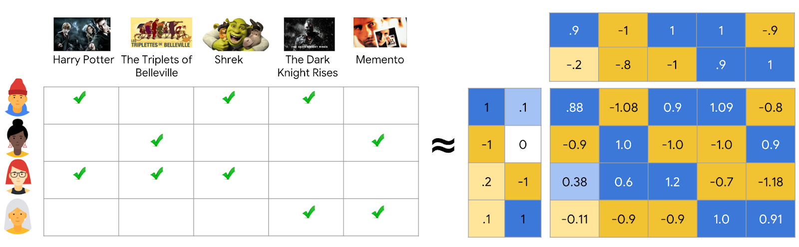
Fig 3. The user-item interaction matrix can be decomposed into a user matrix and an item matrix using matrix factorization techniques
Alternating Matrix Factorization: It uses matrix factorization where you try to represent the user-item interaction matrix as two matrices - a user matrix which describes what the user likes and an item matrix which represents what the item is about (or that is what we assume these matrices represents, you can also think that we are breaking down a single big matrix into the product of two smaller matrices). It’s hard to estimate both matrices at the same time because they depend on each other. So instead, iALS breaks the problem into two steps and repeats them:
First, it fixes the item matrix and calculates the best user preferences that help estimate the user-item interaction data
Then, it fixes the user preferences and calculates the best item features that estimate the user-item interaction data.
By switching back and forth—alternating between updating users and items—it gradually improves both until the model fits the data well.
Fills in the blanks smartly: Even if a user hasn’t listened to most songs, iALS still considers those "missing" interactions. It assumes that the absence of interaction is weak negative feedback, not that the user dislikes it, but just that we have lower confidence.
So let's try out building it. First, let's grab the ‘listens’ dataset from Yambda, which acts as ‘implicit‘ feedback, since the user is taking any specific action to let us know that they liked the song.
# using implicit signals i.e. listens
# Note: Takes ~17m while to load (use dask?)

listens = pd.DataFrame(load_dataset("yandex/yambda", data_dir="flat/50m", data_files="listens.parquet")['train'])
listens.head()
We see that it has `played_ratio_pct`, which has a value between 0-100. Let’s assume that if the user listened to at least 50% of the song, then they probably like the song. We can use this to create a binary implicit signal and create our train/test sets.
Let’s also aggregate all these binary signals together so that if a user listened to more than 50% song, say five times, then the score would be 5.
# Split the data
train_df = listens[listens['timestamp'] <= TRAIN_TIMESTAMP]
train_df = train_df.groupby(['uid','item_id'])['timestamp'].count().reset_index()

test_df = listens[listens['timestamp'] > TEST_TIMESTAMP]
Next, let's process the train dataset to create a user-interaction matrix, and since it tends to be huge, we use scipy csr/coo matrices to keep memory requirements down
# Map user/item IDs to integer indices
user_id_map = {uid: idx for idx, uid in enumerate(train_df["uid"].unique())}
item_id_map = {iid: idx for idx, iid in enumerate(train_df["item_id"].unique())}

train_df["uid_idx"] = train_df["uid"].map(user_id_map)
train_df["item_idx"] = train_df["item_id"].map(item_id_map)
rows = train_df["uid_idx"].values
cols = train_df["item_idx"].values
data = train_df["timestamp"].values

user_item_matrix = coo_matrix((data, (rows, cols)))
user_item_matrix = user_item_matrix.tocsr()
Next, let’s build the ALS model. The model does have a few hyperparameters to tune, but to keep this post short, we are gonna go with a few common starter parameters.
Aside: Hyperparameter for ALS (from implicit python package)
factors (latent dimensions):
Higher values increase model complexity, reducing bias but increasing variance and training time. Too high can lead to overfitting and slower performance.regualarization
Controls overfitting. Higher regularization increases bias (simpler model), reduces variance, and usually improves generalization. Too low can cause overfitting, especially with sparse data.iterations
Number of ALS optimization steps. More iterations reduce bias by improving convergence but increase training time. Diminishing returns after a point.alpha
Scales confidence in observed interactions. Higher alpha reduces bias by weighting observed interactions more, but increases variance and training instability if too high.
Please note that hyperparameter tuning is expected for a production model.
model = AlternatingLeastSquares(factors=64, regularization=0.05, iterations=15, alpha=1, random_state=42)
model.fit(user_item_matrix)
Now, the evaluation. Let’s focus on onlythe user and items we have seen in training, and use the recommend method within implicit to get the top-k recommendation
# filter to relevant set (Note: this means we dont evaluate for cold-start)

test_df = test_df[test_df["uid"].isin(user_id_map)]
test_df = test_df[test_df["item_id"].isin(item_id_map)]

test_df["user_idx"] = test_df["uid"].map(user_id_map)
test_df["item_idx"] = test_df["item_id"].map(item_id_map)

test_df = test_df.dropna(subset=["user_idx", "item_idx"]).astype({"user_idx": int, "item_idx": int})

# this create items 'listened' by each user
user_to_liked_items = defaultdict(set)
for _, row in test_df.iterrows():
    user_to_liked_items[row["user_idx"]].add(row["item_idx"])


# to evaluate the model results
def evaluate_als(model, user_item_matrix, user_to_liked_items, k=10):
    recall_list = []
    ndcg_list = []

    for user_idx, liked_items in user_to_liked_items.items():

        # Get top-K ALS recommendations (filtering known training items)
        recommended = model.recommend(user_idx, user_item_matrix[user_idx], N=k, filter_already_liked_items=False)
        rec_items, _  = recommended

        recall = recall_at_k(rec_items, liked_items, k)
        ndcg = ndcg_at_k(rec_items, liked_items, k)

        if recall is not None:
            recall_list.append(recall)
        if ndcg is not None:
            ndcg_list.append(ndcg)

    return {
        "Recall@K": np.mean(recall_list),
        "NDCG@K": np.mean(ndcg_list)
    }

# Evaluate ALS model
results = evaluate_als(model, user_item_matrix, user_to_liked_items, k=10)
print(f"Recall@10: {results['Recall@K']:.4f}")
print(f"NDCG@10: {results['NDCG@K']:.4f}")
The output is:
Recall@10: 0.0172
NDCG@10: 0.0387The implicit feedback performs better than the popularity model. This is because the amount of implicit feedback data far exceeds the explicit feedback data, and this shows the value in tracking implicit signals provided by users.
Note: The paper uses Hyperparameter tuning to figure out better parameters for iALS, and achieves a different performance. So, make sure to try out HP tuning!
Let's see if we can fix it by mixing implicit and explicit together.
Mixing Implicit and Explicit Signals
Now, let’s see if we can combine implicit signals, i.e, listens, with explicit signals.
The disadvantage of implicit signals is that they provide no negative feedback. We can account for this by tapping into the dislikes data in Yambda!
So let’s combine both these datasets
dislikes = pd.DataFrame(load_dataset("yandex/yambda", data_dir="flat/50m", data_files="dislikes.parquet")['train'])
train_df_dislike = dislikes[dislikes['timestamp'] <= TRAIN_TIMESTAMP].groupby(['uid','item_id'])['timestamp'].count().reset_index()
train_df_dislike['timestamp'] = - train_df_dislike['timestamp']


# iALS using Listen+ | Split the data
train_df = listens[listens['timestamp'] <= TRAIN_TIMESTAMP]
train_df = train_df.groupby(['uid','item_id'])['timestamp'].count().reset_index()

train_df = pd.merge(train_df, train_df_dislike, how='outer', on = ['uid','item_id']).fillna(0)
train_df['conf'] = train_df['timestamp_x'] + train_df['timestamp_y']
train_df = train_df[['uid','item_id','conf']]
Next, we build the model and evaluate the performance
# Map user/item IDs to integer indices
user_id_map = {uid: idx for idx, uid in enumerate(train_df["uid"].unique())}
item_id_map = {iid: idx for idx, iid in enumerate(train_df["item_id"].unique())}

train_df["uid_idx"] = train_df["uid"].map(user_id_map)
train_df["item_idx"] = train_df["item_id"].map(item_id_map)
rows = train_df["uid_idx"].values
cols = train_df["item_idx"].values
data = train_df['conf'].values

user_item_matrix = coo_matrix((data, (rows, cols)))
user_item_matrix = user_item_matrix.tocsr()

model = AlternatingLeastSquares(factors=64, regularization=0.05, iterations=15, alpha=1, random_state=42)
model.fit(user_item_matrix)

# get user listend items
test_df = listens[listens['timestamp'] > TEST_TIMESTAMP]

test_df = test_df[test_df["uid"].isin(user_id_map)]
test_df = test_df[test_df["item_id"].isin(item_id_map)]

test_df["user_idx"] = test_df["uid"].map(user_id_map)
test_df["item_idx"] = test_df["item_id"].map(item_id_map)

test_df = test_df.dropna(subset=["user_idx", "item_idx"]).astype({"user_idx": int, "item_idx": int})

user_to_liked_items = defaultdict(set)
for _, row in test_df.iterrows():
    user_to_liked_items[row["user_idx"]].add(row["item_idx"])


def evaluate_als(model, user_item_matrix, user_to_liked_items, k=10):
    recall_list = []
    ndcg_list = []

    for user_idx, liked_items in user_to_liked_items.items():

        # Get top-K ALS recommendations (filtering known training items)
        recommended = model.recommend(user_idx, user_item_matrix[user_idx],
                                    N=k, filter_already_liked_items=False)
        rec_items, _  = recommended

        recall = recall_at_k(rec_items, liked_items, k)
        ndcg = ndcg_at_k(rec_items, liked_items, k)

        if recall is not None:
            recall_list.append(recall)
        if ndcg is not None:
            ndcg_list.append(ndcg)

    return {
        "Recall@K": np.mean(recall_list),
        "NDCG@K": np.mean(ndcg_list)
    }

# Evaluate ALS model
results = evaluate_als(model, user_item_matrix, user_to_liked_items, k=10)
print(f"Recall@10: {results['Recall@K']:.4f}")
print(f"NDCG@10: {results['NDCG@K']:.4f}")
Output:
Recall@10: 0.0173
NDCG@10: 0.0389The performance does move up a bit, but not significantly. We could be on the right track. This is where clever feature engineering comes into play. Ask yourself, is a dislike equivalent to a user listening to at least 50% of a song? Should we weigh it more?
Try it out and comment on how the performance changes. Make sure to drop a follow to see what can be done to improve performance.
So What's Next!
To be able to put this project on your resume, you can dive deeper in a few ways
Improve on the iALS model by leveraging more of the data (dislikes/ unlikes/ undislikes).
Consider different heuristics! An interesting paper to check out would be - https://arxiv.org/pdf/2110.14037
Consider building out a two-tower neural network ranking model using the audio embedding and interaction feature, post an iALS candidate generation phase (i.e., let iALS give you, say, 1000 items to recommend, the two-tower model will give the top 10)
To build out these projects, make sure to check out Yambda today - https://bit.ly/4604AH9
Also, if you wanna see any of the above tutorials, leave a like/comment!